
Improving the Classifier Performance in Motor Imagery Task Classification: What are the steps in the classification process that we should worry about?
- DOI
- 10.2991/ijcis.11.1.95How to use a DOI?
- Keywords
- Brain Computer Interface Systems; Motor Imagery Tasks; Pattern Recognition; Machine Learning
- Abstract
Brain-Computer Interface systems based on motor imagery are able to identify an individual’s intent to initiate control through the classification of encephalography patterns. Correctly classifying such patterns is instrumental and strongly depends in a robust machine learning block that is able to properly process the features extracted from a subject’s encephalograms. The main objective of this work is to provide an overall view on machine learning stages, aiming to answer the following question: “What are the steps in the classification process that we should worry about?”. The obtained results suggest that future research in the field should focus on two main aspects: exploring techniques for dimensionality reduction, in particular, supervised linear approaches, and evaluating adequate validation schemes to allow a more precise interpretation of results.
- Copyright
- © 2018, the Authors. Published by Atlantis Press.
- Open Access
- This is an open access article under the CC BY-NC license (http://creativecommons.org/licences/by-nc/4.0/).
1. Introduction
A Brain-Computer Interface (BCI) is a communication system that uses electroencephalography (EEG) signals to extract, decode and translate intentions into commands. When they first were developed, the may purpose of BCI systems was to enable the interaction of severe motor disabled people with devices such as computers, speech synthesisers or neural prostheses, which gave the chance for tetraplegic people, individuals with amyotrophic lateral sclerosis, brain stem stroke or spinal cord injury to achieve a higher independence status, improving their quality of life. Today, there are many applications for BCI to control external devices such as robots, communication systems, games, virtual reality or rehabilitative applications 1,2. BCIs are also applied to user-state monitoring or for the evaluation of neuro-marketing applications, in training or education programs, for cognitive improvement or in safety and security applications 2. In summary, these systems detect specific patterns of a person’s EEG that relate to their intentions to initiate control and translate them into meaningful control commands. The detection of these patterns is crucial and depends on a strong component of signal processing and classification.
Typically, a BCI system (Fig. 1) can be seen as an artificial intelligence system 3 that follows five consecutive stages: a) EEG signal generation, b) EEG signal acquisition and preprocessing, c) Feature Extraction, d) Classification and finally e) Applications. Although all parts are important in BCI systems, it is obvious that a good design of the machine learning block is necessary to obtain a good performance. Into the bargain, the quality of predictions depends on both the extracted features and the classification algorithm employed. Several different methods can be applied to extract features from channels located at specific brain areas, such as Spectral Parameters, Parametric Modelling, Signal Envelope, Signal Complexity or some combination of different feature extraction methods 1,3,4,5. Thus, classification algorithms have to manage large feature vectors even when the information provided by some features is not relevant and it increases the complexity of the classifier design. Therefore, as it is shown in the literature, researchers have applied Feature Selection (FS) techniques such us Genetic Algorithms or Feature Transformation (FT) approaches such as Principal Component Analysis (PCA), Independent Component Analysis (ICA), or Common Spatial Patterns (CSP) 1,6,7,8 in order to get the most discriminative features. Also, linear classifiers, neural networks, nonlinear Bayesian classifiers, nearest neighbour and combinations of them 1,3 have been tested, under different sampling strategies, to improve the classification accuracy results. However, there is not a conclusion about which is the best way to design the machine learning stage since each author decides which steps and techniques to apply in each work.
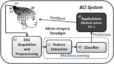
General scheme of a BCI system.
There are different control signal types in BCI: visual evoked potentials, slow cortical potentials, P300 evoked potentials, and sensorimotor rhythms1. One of the most widely studied EEG-based BCI paradigms is the motor-imagery-based BCI 9. Motor Imagery (MI) is defined as an imagining of kinesthetics movements, and it is well known to modulate sensorimotor rhythm around the motor cortex 10.
In this work, EEG signals acquired under MI paradigms have been processed. These are BCI signals from BCI competitions II and III, which represent standard datasets to test signal processing methods and algorithms. The overall goal of this work is to study several pattern recognition approaches able to select/extract relevant features from BCI datasets and identify the patterns that correspond to an individual’s intent of initiating control (a binary classification problem). Thus, stages (c) and (d) will be analysed in a deeper way in order to answer this question: “What are the steps in the classification process that we should worry about?”.
The contribution of this research is therefore two-fold: for researchers familiarised with the field, it provides a comprehensive comparison of approaches included in several stages of the machine learning block comprised in BCI systems; for researchers new to the field, it provides an extensive description and illustration of a complete experimental setup in BCI domains, from the data collection stage to the final classification task, including a thorough explanation of all the techniques frequently used along the process.
The manuscript is organised as follows. Section 2 covers the experimental setup and a brief background on the algorithms used in this work. Section 3 presents and discusses the obtained results. Finally, in Section 4 some conclusions and future directions are discussed.
2. Experimental Setup
In this work, in order to reflect the most usual steps applied from a machine learning perspective in BCI systems, the Machine Learning block has been expanded in six different stages: 1) Feature Computation, 2) Feature Preprocessing, 3) Feature Selection, 4) Feature Transformation/Projection, 5) Classification Task and finally 6) Performance Evaluation (Fig. 2). Stages 1 and 2 consider the implementation of well-established approaches to BCI data, in what concerns feature extraction (Power Spectrum Density, Hjorth Parameters and Adaptive and Autoregressive Parameters) and feature preprocessing (Z-score normalisation). This work mainly investigates concurring approaches from stages 3 to 6, where several different techniques are compared: in stage 3, five techniques have been tested for feature selection (Area Under the ROC Curve, Fisher Score, Information Gain, Point Biserial Correlation and Kruskal-Wallis test); in stage 4, three methods were studied for feature transformation (Principal Component Analysis, Linear Discriminant Analysis and Isomap); in stage 5, four different machine learning classifiers were considered (Fisher Linear Discriminant, Naïve Bayes, Support Vector Machines and Decision Trees) and finally, in stage 6, three validation methods were applied (Holdout, k-fold cross-validation and Leave-One-Out). The main aspects of each stage are discussed below.
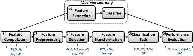
Proposed experimental setup.
2.1. Data Description and Feature Computation
This work focuses on the labeled data of four BCI datasets from four different subjects (Table 1). The data comes from “BCI Competitions” that are widely known in BCI research. The goal of these competitions is to validate signal processing and classification methods for Brain Computer Interfaces (BCIs) 11.
| Subject | Dataset origin | Trials | Classes | Feedback |
|---|---|---|---|---|
| 1 | BCI comp. II | 140 | 2 | Bar |
| 2 | BCI comp. III | 320 | 2 | Basket |
| 3 | BCI comp. III | 540 | 2 | Basket |
| 4 | BCI comp. III | 540 | 2 | Bar |
Dataset description for all 4 subjects.
All the signals used in this work were collected with a g.tec amplifier working at 128 Hz, under a MI paradigm: in particular, the movement of right (RH) or left hand (LH). In all experiments, three bipolar channels located over C3, Cz and C4 were used, although only signals from C3 and C4 filtered between 0.5 and 30Hz were chosen to compute the feedback signals. The data of Subject 1 has been extracted from BCI Competition II (set III). In this experiment, the subject was relaxed in a chair looking at a screen: each trial started with a black screen and two seconds later, an acoustic signal marked the beginning of the trial (Fig. 3). Then, a cross appeared during one second and an arrow (left or right) was displayed as a cue. At this moment, the user imagined the movement of the corresponding hand to move a bar into the direction of the cue. The bar reflects the real time output of the classifier along the feedback period and it was computed based on adaptive autoregressive parameters (AAR) and a discriminant analysis 11.
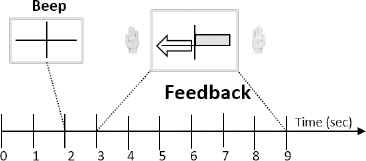
Timing of bar feedback: BCI Competition II, set III.
The data from the 2nd, 3rd and 4th subjects comes from BCI competition III (set IIIb). For this experiment, the timing and the feedback was slightly different. In the beginning of each trial, the screen was black until a cross appeared after two seconds. Then, an acoustic signal attracted the user’s attention, a visual cue appeared and feedback started. Subjects 2 and 3 used basket feedback (Fig. 4) computed with AAR and an adaptive quadratic discriminant analysis. Basket feedback consisted of a ball falling down from the centre top of the screen, and the user should try to move the ball to the left or right depending on its colour (green for left or red for right). Subject 4 used also a bar feedback computed using alpha and beta band power and a linear discriminant analysis.12.
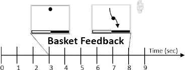
Timing of basket feedback: BCI Competition III, set IIIb.
In order to take advantage of the complementary information provided by different feature extraction methods, for all subjects three feature Extraction methods have been applied in channels C3 and C4: Power Spectral Density (PSD) in alpha and beta frequency bands, Hjorth parameters (Activity, Mobility and Complexity), Auto Regressive (AR) model coefficients of six order and Continuous Wavelet Transform coefficients (CWT) using a standard “Daubechies D2” wavelet type with six features per channel, as done in previous works. 8,13,14. These FE methods have been widely applied in BCI systems and they are very representative of MI tasks4. Features have been computed in a standard 1 second window in the MI period 3, and therefore, there is a vector with 34 features per trial. It is important to remark that the analysis of the feature computation is not the objective of this work.
2.2. Feature Preprocessing
Data preprocessing is performed to reduce noise and increase the consistency of data. The most common preprocessing steps used in the literature are Normalisation or Standardisation of data. Normalisation (Min-Max transformation) refers to the feature scaling between its minimum and maximum values, while Standardisation (Z-Score transformation) transforms the features so that they have a zero mean and unitary standard deviation. The objective of normalisation/standardisation is to make features with different scales and ranges of measurement comparable, so that none has more influence than the others on classification task. In this work, the Z-Score transformation (equation 1) 15 was applied, which is a common feature processing algorithm for BCI 14. In equation 1, xi is each value from a given feature, and µ and σ are the mean and standard deviation of such feature, respectively. Z-score is applied as a standard procedure for data cleaning 16,17, since this stage is not the main focus of our analysis.
2.3. Feature Selection
After preprocessing, a common procedure is to reduce the dimensionality of the input data in order to ease the classification task. This can be done by assessing the discriminative quality of the input features, called Feature Selection (FS), or by Feature Transformation (FT), where the input data is projected onto a low dimensional space 18,19,20,21. FS techniques keep the original meaning of the input features, thus providing a good interpretation of the low-dimensional space: the selected features will be a set of the most discriminative and relevant features for the MI problem. Besides, once the most discriminative features are determined, only them need to be computed for new subjects. In this paper we have computed five FS techniques: AUC values, F-score, IG, rpb and KW. These approaches are representative from a machine learning perspective and they have been previously used in BCI systems 7,22,23,24,25,26. We now describe the different FS techniques explored in this work.
2.3.1. AUC values
The Area Under the ROC curve (AUC) is most often used as performance measure for classification. The Receiver Operating Characteristics curve (ROC) is a plot that represents the trade-offs between the classifier’s true positive rate (TPR) in the yy axis, and false positive rate (FPR) in the xx axis and thus it informs on the variation of the classifier’s sensitivity and specificity for different cut-off values (classification thresholds) 27. Given that both TPR and FPR range from 0 to 1, the AUC of an ideal classifier is 1. Therefore, the discriminant power of a classifier is associated to the area under that curve: the higher the area is, the better. However, the AUC can also be used to determine the discriminative power of the existing features: instead of the classifier outputs (scores), the feature values are used to build the ROC curve. Just the same, the bigger the AUC is, the more discriminative the feature is.
2.3.2. F-score
The Fisher score (F-score) is one of the most widely used supervised feature selection methods, and measures the overlap between individual feature values of different classes (RH, LH), where higher values indicate more discriminative features 28. Considering two classes RH and LH, the Fisher score of a feature j is given by equation 2, where µRH, j, µLH, j, σRH, j and σLH,j are the means and standard deviations of classes RH and LH, respective to the j-th feature.
2.3.3. Information Gain
Information Gain (IG) measures the ability of a given feature to discriminate the input patterns (trials), according to their target (RH, LH) 29. It is an entropy-based measure, most often used for selecting the best features at each step in growing a decision tree (e.g. ID3 algorithm). Considering a collection of trials D, containing examples of RH and LH movements, the necessary information to classify a trial in D is defined as I(D), or E(D) (the entropy of D), which measures the impurity of the collection D. E(D) would be 0 if all trials in D belonged to the same class, and 1 if RH and LH were equally represented. Establishing entropy as a definition of impurity, we can measure the effectiveness of a feature j to discriminate classes RH and LH, by computing the entropy of D after using feature j to divide D in several partitions, E(D, j). The effectiveness of a feature (its discriminative power) is therefore given by equation 3 . The top discriminative features are determined by ranking their information gains, for all features in the dataset.
2.3.4. Point Biserial Correlation
The Point Biserial correlation coefficient (rpb) is the most appropriate correlation index between a continuous (interval or ratio-scaled) feature and a dichotomous (binary) feature 30. Considering the motor imagery problem in this work, rpb can be used to assess the discriminative power of each feature j, by determining its correlation with the class label (RH, LH): rpb varies from 0 to 1, where 0 indicates that there is no correlation and 1 indicates an elevated degree of correlation. The point-biserial correlation of each feature can be computed using equation 4 , where µRH, j and µLH,j are the means of feature j for all RH and LH trials, respectively; σj is the standard deviation of feature j; nRH and nLH are the number of trials belonging to RH and LH classes and n is the total number of trials.
2.3.5. Kruskal-Wallis Test
The Kruskal-Wallis (KW) test is a non-parametric test used to compare the distribution of two or more features observed in two or more independent samples. It can be used to test if two or more samples come from the same population or from different populations; in other words, if the samples come from populations with the same distribution 31. The Qui2 values are a result of KW statistics and can be used to rank the features according to their discriminative power: the higher the Qui2 value, the more discriminative the feature is.
2.4. Feature Transformation
Instead of selecting a subset of the most discriminative features, Feature Transformation (FT) methods are able to “combine” the features and project the data onto a different coordinate system, in such a way that the redundancy between features is minimised, and only relevant information is kept. This ability to “combine” the input features, as a higher level of feature fusion, usually increases the classification accuracy 14, which makes FT methods so attractive. However, the data dimensions in the low dimensional space are the result of a combination of the original dimensions (features), which means that the new dimensions (components) do not have any physical interpretation in the problem under study. In this work, three commonly used FT methods in BCI applications are studied 1,32: Principal Component Analysis, Linear Discriminant Analysis and Isomap, described herein.
2.4.1. Principal Component Analysis
Principal Component Analysis (PCA) is an linear, unsupervised dimensionality reduction method, whose objective is to produce a low-dimensional representation of the original input space 14. PCA transforms the set of p correlated original features {x1 ,x2, …, xp} in a smaller set of uncorrelated, orthogonal variables, referred to as principal components (not to be confused with features), {z1, z2, …, zp}. The main idea of PCA is to find an orthonormal transformation to provide the best set of projections (i.e. eigenvectors) to represent the structure of data, with the minimum possible redundancy, but without significant loss of information. The projections are chosen in order to retain the maximum amount of information, measured in terms of data variance: the first component explains the maximum variance in data, the second the following maximum variance and so forth (the last component will be the one that contributes the less to explain the total variance in data). There are two main criteria to choose the optimal number of principal components to keep33: Kaiser criterion and Scree test. Kaiser criterion suggests keeping only components with eigenvalues equal or higher than 1, while the Scree test is based on a plot of the explained variance for each component: it suggests discarding the components starting where the plot levels off. Both criteria are standard approaches for BCI domains 34,35 and were therefore tested in this work.
2.4.2. Linear Discriminant Analysis
Linear Discriminant Analysis (LDA), also called FDA (Fisher Discriminant Analysis) or FLD (Fisher Linear Discriminant) is also a linear transformation technique; yet, while PCA is an unsupervised method, more oriented to feature discrimination and visualisation, LDA is a supervised method that considers class-membership information for data reduction, thus more helpful in data classification 14. LDA is based on the concept of searching for a linear combination of features that allows the maximisation of between-class variance, while minimising the within-class variance. It is important to mention that, while PCA produces a n × p matrix (n being the number of existing patterns and p the number of components), LDA produces a n × 1 vector, where the input space is projected down to one dimension. Although LDA/FDA is a popular method for dimensionality reduction, it can also be used for classification 36. In the context of BCI, this would imply choosing a threshold ω0 such that if the one-dimensional projection of a trial xi, here referred as zi, is higher or equal to ω0, then xi belongs to class RH, and to LH otherwise (zi < ω0 ). Note that, in this work, FLD is not coupled with LDA in the experiments because they give equivalent solutions.
2.4.3. Isomap
Given that PCA and LDA are linear transformations, they may not appropriately reflect nonlinear properties of the data, which constitutes their main disadvantage. Unlike these classical techniques, Isomap is able to discover nonlinear properties underlying the data 37. Isomap is based on three main steps: in the first step, this algorithm takes the input distances dx(i, j) between all pairs i, j from N data points in the high-dimensional input space X, measured either in the standard euclidean metric or in some domain-specific metric. Based on the distances dx(i, j), Isomap determines which points are neighbours on the manifold M, using one of two methods: (i) connecting all points within a fixed radius ɛ or (ii) connecting all points to all of its k nearest neighbours. Then, these relations are represented as a weighted graph G. In the second step, Isomap computes the geodesic distances dM(i, j) between all pairs of points in the manifold M by determining their shortest path distances in the graph G. Finally, Isomap applies the classical Multi-Dimensional Scaling (MDS) to build a matrix of graph distances, constructing a final embedding of the data in a d-dimensional Euclidean space Y that best preserves the estimated intrinsic geometry of data. Similarly to PCA, the intrinsic dimensionality of the data can be estimated by looking for the “elbow” at which the plot of the residual variance of Isomap’s dimensions ceases to decrease significantly with added dimensions. To conduct the experiments in this work, the euclidean distance was used as the input-space distance and the k parameter was chosen to build the graph. The choice of k was set to find the smallest value that still leads to an overall connected graph for each dataset.
2.5. Classification Task
In this stage, the datasets constructed in the previous phases (FS and FT) are tested with four different classifiers previously used in BCI systems in order to compare results: LDA (or Fisher Linear Discriminant, FLD), Naïve Bayes, Support Vector Machines and Decision Trees 1,38,39. LDA/FLD was already described in the previous section, therefore, the following subsections refer to the remaining classifiers.
2.5.1. Naïve Bayes
Naive Bayes (NB) classifier outputs its predictions based on the posterior probabilities of each existing class, P(ωi | x): the probability that pattern x belongs to class ωi40. In a motor imagery task, two posterior probabilities are considered: the probability that a trial x represents a RH movement (ωi = RH), or a LH movement (ωi = LH). NB classifier then calculates these posterior probabilities using equation 5 , where P(ωi) is the prior probability of class ωi, i.e., the probability of occurrence of each class (e.g., proportion of trials that belong to classes RH or LH); p(x | ωi) is called the likelihood of x, which is determined for all feature values in x, given that x is a d-dimensional pattern x= [x1,x2, ..., xd]: the likelihood of x is computed through a multiplication of all these individual likelihoods. Finally, p(x) is the total probability of x, and may be determined using equation 6 , although it can be ignored because it is the same for both classes, due to the sum over all classes.
Given a trial x, NB proceeds to the computation of its posterior probabilities, P(RH | x) and P(LH | x), and decides on the output based on the maximum posterior probability, that is, if P(RH | x) > P(LH | x), then the trial belongs to RH, and to LH otherwise. If the posterior probabilities are equal, then the choice is arbitrary.
2.5.2. Support Vector Machines
The concept behind Support Vector Machines (SVM) is to find a discriminant function that maximises the margin of separation between the existing classes (optimal hyperplane), using the information provided by the boundary patterns (called the support vectors) 41. Considering a motor imagery scenario, where RH and LH classes are linearly separable, the equation of a discriminant hyperplane (decision boundary) would be given by equation 7 , where g(xi) is the classification label, and w and b are the parameters of the hyperplane (weights and bias that define the plane).
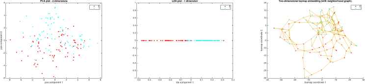
Feature Transformation techniques for subject 1: PCA, LDA and Isomap embedding. PCA shows a two-dimensional scatter plot considering the two most significant principal components in the transformed space; LDA projects the original data into one dimension, the component that guarantees the highest separability between classes, where the helpfulness for classification is clear; Isomap embedding, where each data point (trial) is connected to its two closest neighbours. Input vector from classes RH and LH are denoted as classes 1/0, marked in blue/red circles.
The values of w and b are not unique, and there are an infinity of hyperplanes that could divide classes RH and LH; however, to provide a good generalisation, SVM need to find the optimal hyperplane, the one that maximises the margin separation between the two classes. Defining classes yi = {RH, LH} as yi = {1, −1}, the decision rule is defined by equation 8, and the margin is defined as
2.5.3. Decision Trees
As the name implies, Decision Trees (DT) are supervised, tree-based models, where the input space (all existing BCI trials) is recursively divided into two or more subspaces based on the discriminative power of the existing features 42. A decision tree starts with a root node, which is the feature whose split is more informative for class assignment (e.g. Hjorth activity parameter), and from the root node several branches arise, creating several other nodes, called internal or test nodes. Each node in the tree is a feature (e.g. power spectral density of alpha band in channel 1, adaptive regression model coefficients in channel 2) and represents a condition that must be tested. Branches are the possible solutions for the test conditions at each node, represented by each node’s possible values (for discrete features, they are all the existing categories in the considered subspace; for continuous features, which is the case of this BCI task, each branch represents a certain range of values). The classification of a trial x is achieved by following its path along the nodes, from the root to a terminal node (leaf), according to the conditions tested along the way. Leaves are nodes with only incoming branches (they are not further divided), each one assigned to a class - typically, each leaf assumes the class with the highest fraction of patterns included in its subspace: for instance, a trial that ends in a leaf with 6/10 RH examples and 4/10 LH examples will be assigned to RH class.
2.6. Sampling Strategies
To estimate the performance of a classifier, it’s necessary to determine its error rate across the entire population of examples, which is impractical in real-world applications (the whole population is not available to study). Sampling strategies allow the partition of the existing examples to train and test the classification models, and provide an estimate of the true error. Considering a motor imagery context, these approaches split a subject’s trials into two groups of examples: training examples, where a percentage of trials is used to build the classification model and the test examples, where trials never seen by the model are used for evaluation. In this section, we review the most commonly used strategies in BCI scenarios 43,44,45,46.
2.6.1. Holdout method
Holdout method randomly divides the dataset in k = 2 sets, typically considering a 70%–30% or 80%–20% split for training/test 47. The model is constructed using the training set while the performance metrics are computed using the test set. This method is rather simple, yet comprises some limitations: holdout may be subjected to “unlucky” splits, where the training set may not be representative of the total examples 36.
2.6.2. K-fold cross-validation
In k-fold cross-validation, the dataset is partitioned in k distinct folds, where generally k is commonly set to 10 33. These folds will rotate in such a way that all of them are used for training and testing the model: k − 1 folds are used as training set and the remaining fold (test set) for evaluation, and the procedure is performed k times, rotating the position of the test set. The final error estimation is produced according to equation 10, by averaging the individual errors ei of each fold. This work considers a 10-fold cross-validation scheme. The trade-off between bias and variance of a classifier is influenced by the choice of k: a small k provides a larger bias but low variance, whereas a larger k produces error estimates closer to the true error (low bias), although increasing the variance.
2.6.3. Leave-One-Out
When k = N (with N total examples), the sampling scheme is called Leave-One-Out (LOO), where the model is designed using N − 1 examples and tested using the left-out example, and the process is repeated N times. Thus, the final error estimate is computed by averaging all the N individual errors. LOO uses only one example for testing, which produces a large variance in the error estimation; however, since all the remaining N −1 examples are used for the design of the classifier, the average test error estimate (over all N runs), is an accurate estimate of the true error, resulting in a low bias.
2.7. Performance Evaluation
In BCI contexts, accuracy is the most commonly used metric to evaluate the performance of a classification approach 8,14 and represents the rate of correctly classified patterns. There are, however, several other important metrics to properly evaluate a given approach, and they are, as Accuracy, based on a confusion matrix (Table 2) 48. A confusion matrix describes the performance of a classifier on the basis of its predictions (Predicted Class), versus the true, known classes (Actual Class). Table 2 shows a confusion matrix for binary classification problem, such as the motor imagery task in this work, where “movement of right hand” (RH) is considered the positive class and “movement of left hand” (LH) the negative class. In what follows, we provide a brief explanation of the current performance measures used in MI tasks 49,50.
| Actual | |||
|---|---|---|---|
| Negative | Positive | ||
| Predicted | Negative | True Negative (TN) | False Negative (FN) |
| Positive | False Positive (FP) | True Positive (TP) | |
Confusion Matrix
In the context of BCI motor imagery tasks, the entries in the above confusion matrix have the following meaning: True Positives (TP) and True Negatives (TN) represent the number of trials correctly classified as RH and LH movement, respectively. False Positives (FP) are the number of LH trials that are misclassified as RH movement and False Negatives (FN) represent the number of RH trials misclassified as LH movement. For binary classification problems, a confusion matrix is the starting point for the definition of fundamental performance metrics: Accuracy, Sensitivity, Specificity, Precision and Negative Predictive Value. Herein we explain each one with a specific focus on motor imagery tasks.
Accuracy (Acc), as above mentioned, represents the proportion of correctly classified patterns: the proportion of RH and LH movement predictions that were correct (classified as RH and LH trials, respectively), and is calculated using equation 11.
Sensitivity (Sens) reports on the proportion of positive patterns correctly classified; that is; out of all the existing true RH trials, how many were correctly identified (equation 12). Specificity (Spec) is similar, but respects to the negative class: the proportion of LH trials correctly identified (equation 13).
Precision (Prec) represents the proportion of the predicted positive patetrns that were correctly classified: out of all trials predicted as RH movement, the ones that were in fact representing RH movements (equation 14). The Negative Predictive Value or Negative Prediction (PrecNeg), shows how many predicted negative patterns were correctly identified: of all trials predicted as LH movement, how many were in fact LH movement trials (equation 15).
Precision, along with Sensitivity are the two required terms to compute F-measure (equation 16). F-measure balances the trade-off between Precision and Sensitivity, being defined as a weighted measure of both (an “harmonic mean”). In any context, including motor imagery tasks, achieving a high sensitivity and high precision is difficult, and an effort to improve the performance of one causes a performance decrease in the other. For instance, achieving a maximum Sensitivity would be straightforward: the classifier would simply set all labels to “RH”. For maximum Precision, however, the classifier could not account for any false positives (LH trials classified as RH), which is incompatible with setting all trials to RH for maximum Sensitivity. F-measure then traduces the ability of the classifier to provide strong results in both, by using equation 16.
Besides being used for feature selection, AUC values can also be used for evaluating the classification performance, as previously explained.
3. Experiments and Discussion of Results
Fig. 6 gives an overview of the experiments conducted in this work. The datasets with the extracted features (PSD, H, AR and CWT) from the BCI signals of BCI competitions II and III are analysed. In the first step, for each subject, six different datasets were constructed based on the results of FS and FT algorithms: original dataset, FS dataset, PCAKaiser dataset, PCAScree dataset, Isomap dataset and LDA dataset. After that, the datasets were tested with four different classifiers, each using three sampling schemes (note that LDA is not coupled with FLD). Therefore, 252 different combinations are evaluated. The accuracy, sensitivity, specificity, precision, negative precision, F-measure and AUC values were determined for each one of those 252 combinations.
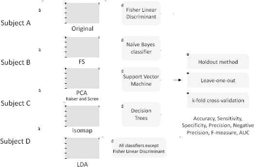
Overview of the experiments.
Since this work comprises an extensive set of simulations, this section will be divided into three main subsections: “Feature Selection Results”, “Feature Transformation Results” and “Classification Results”, to ease the discussion and simplify the analysis by the reader.
3.1. Feature Selection Results
The feature selection results are summarised in Table 3, where each original dataset was analysed to select a subset of the most discriminative features. Considering all subjects, the features related to PSD in the beta frequency, AR and CWT coefficients were the most frequently selected as discriminative. On the contrary, the discriminative power of Hjorth parameters could not be verified for all the subjects. Furthermore, although it is not possible to have the same exact criteria for selection among all subjects, the AUC values, rpb and Qui2 produce similar results, which is important to move towards an approach that returns reliable results, independently of the test subject.
| Subject 1 | Subject 2 | Subject 3 | Subject 4 | |
|---|---|---|---|---|
| AUC | >0.6 | >0.57 | >0.57 | >0.57 |
| F-score | >0.2 | >0.05 | >0.1 | >0.15 |
| IG | >0.1 | >0.02 | >0.02 | >0.02 |
| rpb | >0.2 | >0.15 | >0.2 | >0.2 |
| Qui2 | >10 | >10 | >10 | >10 |
| Selected Features | [1,3], [5,9], [18, 20], 22, [26,28] | [1,3], [6,8], 14, 16, 19, 20, 28 | 2, 4, 12, 21, 29 | 19, [22,28] |
Selected features and criteria used for each dataset.
3.2. Feature Transformation Results
Feature Transformation results are shown in Table 4 and herein explained in what follows. LDA and Kaiser criterion are performed automatically: LDA reduces the input data to one dimension and Kaiser criteria discards principal components with eigenvalues below 1. For the remaining criteria (scree test and isomap embedding), a more thorough analysis is required: the number of components for which the residual variance ceases to decrease significantly needs to be inspected for each subject. Concerning the PCA results, scree test always suggests a higher number of dimensions. In fact, although kaiser criterion keeps the components responsible for the great majority of data variance, there can still be components with low variance that can be helpful for discriminating class-membership. Therefore, scree criteria suggests keeping between 25 to 28 dimensions.
| Subject 1 | Subject 2 | Subject 3 | Subject 4 | |
|---|---|---|---|---|
| LDA | 1 | 1 | 1 | 1 |
| PCAKaiser | 9 | 11 | 11 | 13 |
| PCAScree | 25 | 28 | 26 | 25 |
| Isomap | 6 | 20 | 15 | 25 |
Extracted dimensions for each dataset.
3.3. Classification Results
The classification results are summarised in Table 5 for all subjects. Table 5 presents the results for FLD, NB, SVM and DT using holdout, k-fold cross-validation and LOO: for each type of FS and FT (including also the original dataset), the best value achieved in each performance metric is shown, including the combination of classifier and sampling method that provided such value. In some cases, several classifiers and/or sampling methods are presented, meaning that they achieved the same results. Also, the best value considering all combinations is marked in bold. Overall, FLD and SVM classifiers showed a robust behaviour, being the top two classifiers achieving the highest performance results for the majority of considered combinations. Generally, FS and FT methods seem to improve the baseline classifications (with the original data), with the exception of Isomap embedding, which performs poorly, especially for subjects 3 and 4. The comprehensive set of techniques used for FS achieves better results than PCA and Isomap, although not LDA. Furthermore, the datasets constructed using Scree test returned better results than the ones constructed using the Kaiser criterion, which indicates that for these subjects there are components with low variance that contribute for the discriminative process. Nevertheless, it is LDA that outperforms the remaining FT and FS methods, where an impressive reduction is performed (one dimension). These observations suggest that (i) the combination of the chosen FS methods may be a feasible approach for motor imagery scenarios, with higher performance than other FT methods, (ii) isomap embedding is responsible for the lowest performance, indicating that BCI data benefits the most from linear mappings, such as PCA and LDA, (iii) Scree test maintains several components with low variance that may be crucial for discriminations, and therefore should be preferred over Kaiser criterion, and finally (iv) linear and supervised FT approaches (LDA) are the most appropriate for BCI data, achieving good performance indicators and a considerable reduction of the problem’s dimensionality, decreasing the computational cost of classification tasks.
| Subject 1 | ||||||
| Original | FS | LDA | PCAScree | PCAKaiser | Isomap | |
| Acc | 0.80714 [FLD, LOO] | 0.85714 [DT, Holdout] | 0.92857 [SVM, Holdout] | 0.79286 [FLD, Kfold] | 0.78571 [SVM, Holdout] | 0.78571 [SVM, NB, Holdout] |
| Sens | 0.81429 [NB, Kfold] | 0.85714 [DT, Holdout] | 1 [SVM, NB, Holdout] | 1 [SVM, Holdout] | 0.78571 [FLD, Holdout] | 0.85714 [SVM, Holdout] |
| Spec | 0.81429 [FLD, LOO, Kfold] | 0.92857 [SVM, Holdout] | 0.85714 [SVM, Holdout] | 0.92857 [NB, Holdout] | 0.85714 [SVM, Holdout] | 0.85714 [NB, Holdout] |
| Prec | 0.81159 [FLD, LOO] | 0.9 [SVM, Holdout] | 0.875 [SVM, Holdout] | 0.9 [NB, Holdout] | 0.83333 [SVM, Holdout] | 0.83333 [NB, Holdout] |
| PrecNeg | 0.83548 [FLD, Kfold] | 0.85714 [DT, Holdout] | 1 [SVM, NB, Holdout] | 1 [SVM, Holdout] | 0.77139 [SVM, Kfold] | 0.79476 [SVM, Kfold] |
| Fmeasure | 0.80576 [FLD, LOO] | 0.85714 [DT, Holdout] | 0.93333 [SVM, Holdout] | 0.79452 [FLD, LOO] | 0.76923 [SVM, Holdout] | 0.8 [SVM, Holdout] |
| AUC | 0.87755 [SVM, Kfold] | 0.89388 [SVM, Kfold] | 0.90816 [SVM, Kfold] | 0.88163 [FLD, Kfold] | 0.81633 [FLD, Kfold] | 0.83265 [SVM, Kfold] |
| Subject 2 | ||||||
| Original | FS | LDA | PCAScree | PCAKaiser | Isomap | |
| Acc | 0.67188 [SVM, Holdout] | 0.76562 [FLD, Holdout] | 0.75 [NB, Holdout] | 0.6875 [DT, Holdout] | 0.71875 [SVM, Holdout] | 0.625 [DT, Holdout] |
| Sens | 0.71875 [DT, Holdout] | 0.78125 [FLD, Holdout] | 0.875 [NB, Holdout] | 0.78125 [FLD, Holdout] | 0.65 [DT, LOO] | 0.575 [DT, Kfold] |
| Spec | 0.6875 [DT, Kfold] | 0.75000 [FLD, Holdout] | 0.71875 [DT, Holdout] | 0.675 [FLD, Kfold] | 0.8125 [SVM, Holdout] | 0.71875 [DT, Holdout] |
| Prec | 0.66667 [SVM, Holdout] | 0.75758 [FLD, Holdout] | 0.7 [NB, Holdout] | 0.66667 [DT, Holdout] | 0.76923 [SVM, Holdout] | 0.65385 [DT, Holdout] |
| PrecNeg | 0.67742 [SVM, Holdout] | 0.77419 [FLD, Holdout] | 0.83333 [NB, Holdout] | 0.71429 [DT, Holdout] | 0.68421 [SVM, Holdout] | 0.60526 [DT, Holdout] |
| Fmeasure | 0.67692 [SVM, Holdout] | 0.76923 [FLD, Holdout] | 0.77778 [NB, Holdout] | 0.70588 [DT, Holdout] | 0.68966 [SVM, Holdout] | 0.58621 [DT, Holdout] |
| AUC | 0.68008 [FLD, Kfold] | 0.75039 [DT, Kfold] | 0.77617 [NB, DT, Kfold] | 0.70273 [FLD, Kfold] | 0.69922 [FLD, Kfold] | 0.61484 [DT, Kfold] |
| Subject 3 | ||||||
| Original | FS | LDA | PCAScree | PCAKaiser | Isomap | |
| Acc | 0.76111 [FLD, Kfold] | 0.77778 [NB, Holdout] | 0.81481 [NB, Holdout] | 0.73519 [FLD, LOO] | 0.67778 [FLD, Kfold] | 0.59074 [FLD, Kfold, SVM, LOO] |
| Sens | 0.74815 [FLD, LOO] | 0.77778 [FLD, Holdout] | 0.81481 [NB, Holdout] | 0.71481 [FLD, LOO] | 0.7037 [SVM, LOO, DT, Holdout] | 0.62963 [DT, Holdout] |
| Spec | 0.78519 [FLD, Kfold] | 0.77778 [DT, Holdout] | 0.81481 [NB, Holdout] | 0.75556 [FLD, LOO, SVM, Kfold] | 0.7037 [SVM, Holdout] | 0.59259 [SVM, Holdout] |
| Prec | 0.77692 [FLD, LOO] | 0.75862 [NB, Holdout] | 0.81481 [NB, Holdout] | 0.74517 [FLD, LOO] | 0.68 [SVM, Holdout] | 0.59041 [SVM, LOO] |
| PrecNeg | 0.75714 [FLD, LOO] | 0.8 [NB, Holdout] | 0.81481 [NB, Holdout] | 0.72598 [FLD, LOO] | 0.68779 [SVM, Kfold] | 0.59465 [SVM, Kfold] |
| Fmeasure | 0.76226 [FLD, LOO] | 0.78571 [NB, Holdout] | 0.81481 [NB, Holdout] | 0.72968 [FLD, LOO] | 0.68592 [SVM, LOO] | 0.5915 [SVM, LOO] |
| AUC | 0.82936 [FLD, Kfold] | 0.81427 [SVM, Kfold] | 0.85665 [NB, Kfold] | 0.80055 [FLD, Kfold | 0.71605 [FLD, Kfold] | 0.61619 [FLD, Kfold] |
| Subject 4 | ||||||
| Original | FS | LDA | PCAScree | PCAKaiser | Isomap | |
| Acc | 0.7037 [SVM, Holdout] | 0.69815 [SVM, Kfold] | 0.77778 [NB, Holdout] | 0.73148 [SVM, Holdout] | 0.68519 [FLD, Holdout] | 0.65741 [SVM, Holdout] |
| Sens | 0.66667 [FLD, Holdout] | 0.74074 [FLD, Holdout] | 0.81481 [DT, Holdout] | 0.77778 [SVM, Holdout] | 0.68519 [FLD, Holdout] | 0.61111 [FLD, Holdout] |
| Spec | 0.75926 [SVM, Holdout] | 0.72963 [SVM, Kfold] | 0.81481 [NB, SVM, Holdout] | 0.69519 [SVM, Holdout] | 0.68519 [FLD, Holdout, SVM, Kfold] | 0.81481 [SVM, Holdout] |
| Prec | 0.72917 [SVM, Holdout] | 0.71971 [SVM, Kfold] | 0.8 [NB, Holdout] | 0.71186 [SVM, Holdout] | 0.68519 [FLD, Holdout] | 0.72973 [SVM, Holdout] |
| PrecNeg | 0.68333 [SVM, Holdout] | 0.70213 [FLD, Holdout] | 0.75062 [NB, Holdout] | 0.7551 [SVM, Holdout] | 0.68519 [FLD, Holdout] | 0.61972 [SVM, Holdout] |
| Fmeasure | 0.68627 [SVM, Holdout] | 0.69565 [FLD, Holdout] | 0.76923 [NB, Holdout] | 0.74336 [SVM, Holdout] | 0.68519 [FLD, Holdout] | 0.59341 [SVM, Holdout] |
| AUC | 0.74266 [FLD, Kfold | 0.74966 [FLD, Kfold] | 0.78615 [NB, Kfold] | 0.72195 [FLD, Kfold] | 0.70261 [SVM, Kfold] | 0.6598 [SVM, Holdout] |
Overall performance results.
It must be noted that some improvements in performance are associated with the holdout method; however, the comparison between datasets and classifiers using only this method might not be the most appropriate approach, since different random partitions of data could have different results (“lucky splits” or “unfortunate splits” may happen, as previously explained). For that reason, Table 6 focuses on the results for LOO for all classifiers: since FLD is one of the most extensively used machine learning algorithms in BCI research, the results obtained with FLD and LOO for the original datasets define the baseline classification for this analysis. The feature reduction using LDA, coupled either with NB or SVM, consecutively improved the baseline results for all subjects, which suggests that LDA is a suitable approach for dimensionality reduction in BCI data. DT performed poorly, and thus is not considered to be a valid approach to use on this type of problem. Another observation is that, when considering only the LOO results, SVM is still one of the top classifiers, although it shares its place in the podium with NB classifier, which is increasingly receiving a renewed attention for motor imagery tasks in recent years 3,38.
| Subject 1 | Subject 2 | Subject 3 | Subject 4 | |||||
|---|---|---|---|---|---|---|---|---|
| FDA Baseline | Best Approach | FDA Baseline | Best Approach | FDA Baseline | Best Approach | FDA Baseline | Best Approach | |
| Acc | 0.80714 | 0.817143 [SVM, LDA] | 0.61562 | 0.6875 [NB, LDA] | 0.76667 | 0.77037 [NB, LDA] | 0.67963 | 0.70556 [SVM, LDA] |
| Sens | 0.8 | 0.97143 [SVM, LDA] | 0.63125 | 0.775 [NB, SVM, LDA] | 0.74815 | 0.7963 [NB, LDA] | 0.66296 | 0.75926 [NB, LDA] |
| Spec | 0.81429 | 0.82857 [SVM, FS] | 0.6 | 0.675 [FLD, SVM, FS] | 0.78519 | 0.79259 [SVM, LDA] | 0.6963 | 0.71481 [SVM, FS] |
| Prec | 0.81159 | 0.82278 [NB, LDA] | 0.61212 | 0.66452 [FLD, FS] | 0.77692 | 0.78125 [SVM, LDA] | 0.68582 | 0.69922 [SVM, FS] |
| PrecNeg | 0.80282 | 0.96429 [SVM, LDA] | 0.61935 | 0.72727 [NB, LDA] | 0.75714 | 0.78516 [NB, LDA] | 0.67384 | 0.72917 [NB, LDA] |
| Fmeasure | 0.80576 | 0.88312 [SVM, LDA] | 0.62154 | 0.71264 [NB, LDA] | 0.76226 | 0.77617 [NB, LDA] | 0.6742 | 0.7193 [NB, LDA] |
| AUC | 0.72648 | 0.73643 [NB, LDA] | 0.57532 | 0.61186 [FLD, FS] | 0.69708 | 0.70065 [NB, LDA] | 0.62717 | 0.63695 [SVM, FS] |
Leave-one-out performance results: FDA baseline versus Best Approach.
Furthermore, we also present the k-fold cross-validation accuracy results for the original and LDA reduced datasets, considering all classifiers, in order to assess the variance in the predictions of each classifier (only k-fold provides an estimate on the variance of the predictions, through the standard deviation of the performance achieved in each fold). The k-fold results (Table 7), confirm that transforming the datasets with LDA improves the accuracy results, with also lower standard deviations than for the same approach in the original datasets. BCI datasets can therefore be extremely reduced with LDA without significant loss of information. Furthermore, NB and SVM achieved frequently similar results, although generally SVM results are slightly better.
| Subject 1 | Subject 2 | Subject 3 | Subject 4 | |||||
|---|---|---|---|---|---|---|---|---|
| Original | LDA | Original | LDA | Original | LDA | Original | LDA | |
| FLD | 0.8 ± 0.1338 | n.a. | 0.6062 ± 0.0782 | n.a. | 0.7611 ± 0.0575 | n.a. | 0.6722 ± 0.0912 | n.a. |
| NB | 0.7643 ± 0.1169 | 0.8643 ± 0.0786 | 0.6062 ± 0.1044 | 0.6906 ± 0.1015 | 0.6611 ± 0.0479 | 0.7685 ± 0.0747 | 0.6500 ± 0.0332 | 0.7037 ± 0.0262 |
| SVM | 0.7714 ± 0.0811 | 0.8714 ± 0.0563 | 0.6156 ± 0.1170 | 0.6875 ± 0.0859 | 0.7537 ± 0.0630 | 0.7667 ± 0.0518 | 0.6648 ± 0.0758 | 0.7093 ± 0.0454 |
| DT | 0.7714 ± 0.1421 | 0.8214 ± 0.1078 | 0.6438 ± 0.0886 | 0.6594 ± 0.0772 | 0.6185 ± 0.0574 | 0.7167 ± 0.0531 | 0.6000 ± 0.0820 | 0.6759 ± 0.0587 |
K-fold crossvalidation accuracy results: Original Data versus LDA Projection.
4. Conclusions and Future Work
In this work, a comprehensive study of the stages that compose the machine learning block of BCI systems is performed. Existing approaches applied in several stages – feature selection, feature transformation, classification and performance evaluation – are explained and discussed in detail, in order to address the following research question: “What are the steps in the classification process that we should worry about?”. To that end, a thorough study of four motor imagery datasets was performed. Each dataset was analysed using five methods for feature selection (AUC, F-score, Information Gain, rpb and Qui2), three methods for feature transformation (LDA, PCA with Kaiser and Scree criteria and Isomap), four different classifiers (FLD, NB, SVM and DT) and three sampling strategies (holdout, k-fold cross-validation and leave-one-out), resulting in 252 different combinations (LDA is not coupled with FLD). Regarding the dimensionality reduction of motor imagery dataset, all FS and FT approaches improved the baseline results. The set of FS techniques tested seems to be a feasible approach, where features related to the PSD in the beta bands, and two specific AR and CWT coefficients seem to be the most discriminative for motor imagery tasks. Also, FS seemed to be better for discrimination than some FT techniques, such as PCA and Isomap, although not LDA. In particular, Isomap performed poorly, and does not seem to be an appropriate reduction method for motor imagery. BCI data seems therefore to benefit the most from linear mappings, rather than nonlinear ones, and in particular from linear, supervised methods such as LDA, which has shown very good results. Regarding classifiers, none has strongly outperformed all others for all considered combinations and subjects, although SVM and NB showed a robust behaviour, particularly when coupled with LDA. Regarding the sampling schemes, although LOO produces a better estimate of the true performance error, it has a large variance. On the other hand, k-fold cross-validation, with a proper value of k, is also able to accurately approximate the true error, while providing a meaningful insight on the variance between estimates, which helps in establishing a measure of confidence in the designed classification model.
Facing these results, as a final conclusion of this work, it is clear that future research in this area should focus on transformation techniques for dimensionality reduction, in particular on the development/application of supervised linear approaches. However, a more thorough exploration of Naive Bayes classifiers for motor imagery problems, could also constitute an important contribution for knowledge. Performance results should be evaluated with k-fold cross-validation in order to provide an estimate of how much the classifier varies in its predictions. As a final remark, the validation of these results could benefit from the analysis of different BCI datasets with more subjects and more EEG channels in order to manage higher groups of features in each trial.
Acknowledgments
The authors would like to dedicate this work to the memory of our colleague Professor Pedro J. García-Laencina who sadly passed away during the course of this work.
References
Cite this article
TY  - JOUR
AU  - Miriam Seoane Santos
AU  - Pedro Henriques Abreu
AU  - Rodríguez-Bermúdez Germán
AU  - Pedro J. García-Laencina
PY  - 2018
DA  - 2018/07/26
TI  - Improving the Classifier Performance in Motor Imagery Task Classification: What are the steps in the classification process that we should worry about?
JO  - International Journal of Computational Intelligence Systems
SP  - 1278
EP  - 1293
VL  - 11
IS  - 1
SN  - 1875-6883
UR  - https://doi.org/10.2991/ijcis.11.1.95
DO  - 10.2991/ijcis.11.1.95
ID  - Santos2018
ER  -