
A Robust Predictive–Reactive Allocating Approach, Considering Random Design Change in Complex Product Design Processes
- DOI
- 10.2991/ijcis.11.1.91How to use a DOI?
- Keywords
- robust predictive–reactive allocating; design change; compressing execution time; match-up time
- Abstract
In the highly dynamic complex product design process, task allocations recovered by reactive allocating decisions are usually subject to design changes. In this paper, a robust predictive–reactive allocating approach considering possible disruption times is proposed, so that it can absorb the disruption in the executing process and utilize the limited capacity of resource more effectively. Four indexes (Makespan, stability, robustness, and compression cost) are used to measure the quality of the proposed method. To illustrate the novel allocating idea, we first assign tasks to resources with the objective of a trade-off between the overall execution time and the overall design cost, which can transform the problem into a non-identical parallel environment. Then, the probability distribution sequencing (PDS) method combining with inserting idle time (IIT) is proposed to generate an original-predictive allocation. A match-up time strategy is considered to match up with the initial allocation at some point in the future. The relationship between the minimum match-up time and the compression cost is analyzed to find the optimal match-up time. Our computational results show that the proposed sequencing method is better than the shortest processing time (SPT) which is a common sequencing way mentioned in the literature. The robust predictive–reactive allocating approach is sensitive to the design change, which is helpful to reduce the reallocating cost and keep the robustness and stability.
- Copyright
- © 2018, the Authors. Published by Atlantis Press.
- Open Access
- This is an open access article under the CC BY-NC license (http://creativecommons.org/licences/by-nc/4.0/).
1. Introduction
Complex products such as large technical systems are inherently complex to design. Complex Product Design (CPD) are developed through decomposition into a series of sub-systems and components1, 2. Macroscopically, decomposition creates many interdependencies linking design tasks performed by different designers from different domains which are responsible for the synthesis of solutions for different parts of the system. To guarantee the design process in a controllable state without sufficient knowledge about the imprecision caused by different kinds of design change is the essential issue for the success of CPD.
The existing literature, on problems of task allocating, mainly considers the environments with static and deterministic versions3, 4. However, the actual allocating problem of CPD in real life is dynamic and uncertain2,4, since a design change occurs inevitably and then disrupts the execution of CPD processes. Numerous interdependencies in CPD imply that any design change may trigger arbitrary design variables which could affect or diffuse the degree of uncertainty of the variables that it is connected to. Thus, managing design change is important for decision-makers to carry out a controllable CPD process.
Design change necessitates reallocating the remaining tasks of the initial allocation plan. The high efficiency and timeliness of task allocating are particularly important. To the best of our knowledge, most studies in the literature are based on the exact values of the actual conditions. In a dynamic environment, especially for CPD process, it is difficult to guarantee the precise value of the task execution time, the completion time, and the delivery5. On the other hand, task allocating is flexible and learnable, that is, the execution time is variable and controllable. The controllability of the executing time provides flexibility in reallocating against unexpected design changes by compressing the executing time6. In addition, the existing task allocation strategy concentrates on the coordination efficiency when a design change occurs but lacks the ability to anticipate design change. The performance of reallocating strategies highly depends on the allocation state at the time of disruption7. Under the condition of incompletely accurate information, it is of great practical significance to study the CPD task allocation method which has the ability to predict abnormal factors and processing real-time problems.
Predictive–reactive scheduling is a scheduling/rescheduling process in which schedules are revised in response to real-time events8. The predictive– reactive scheduling strategies are mianly based on simple allocation adjustments which consider only efficiency9. The new schedule may deviate significantly from the original schedule, which can seriously affect other planning activities in the original schedule, and may weaken their performance. Therefore, it is desirable to generate the robust predictive–reactive schedules, to minimize the effects of disruption on the performance of planning activities. A typical solution to generate a robust schedule is to reschedule by simultaneously considering both efficiency and deviation from the original schedule, that is, the stability.
Two kinds of major negative impacts on the original allocations are accompanied by design change. First, it degrades allocation performance. This effect is the topic of robustness. Second, unforeseen design changes cause variability. This effect is the topic of stability. A schedule whose realization does not deviate from the original schedule in the face of disruptions is called stable.
To illustrate the robust predictive–reactive allocating approach with the compressibility of controllable execution time, a task-resource assignment is obtained to transform this problem into a parallel non-identical resources problem firstly. The objective of this problem is to keep the trade-off of the overall execution time and overall design cost. Then, the optimal compression levels on the executing time of the task are estimated to support the task sequencing on each Virtual Design Unit (VDU, which is a specific definition described in Section 3). In this paper, the probability distribution of design change is considered to find the executing sequence on each VDU (we combine the advantages of inserting idle times and controllable executing times). When design change occurs, a match-up time strategy is applied to catch up with the original allocation. In the considered reactive allocating problem, the objective is to minimize the change-adaption cost caused by disruptions, subjected to the condition that the reallocation needs to match up with the original allocation at the match-up time point after disruption10. The performance comparison of the proposed approach and other common approaches in the existing literature is discussed.
2. Literature Review
2.1 Task allocating approach
In the literature of allocating approaches, completely reactive allocating, predictive–reactive allocating, and robust pro-active allocating have been considered extensively11–13. In those studies, the allocation is usually restored within a slight adjustment to the control the performance degradation. Yang et al.14 presented an adaptive task scheduling strategy for heterogeneous Spark cluster, which could analyze parameters from surveillance to adjust the task allocation weights of nodes.Aytug et al.15 gave an extensive literature survey on allocating under uncertainty and generating robust allocations. Fernandes et al.16 presented an imprecision management method to support large organizations for design process management. Salimi et al.17 improved the NSGA-II using fuzzy operators to improve the quality and performance of task scheduling in the market-based grid environment. In their research, the load balancing, Makespan and Price are regarded as the three important objectives for the task scheduling problem. Huang18 proposed a dynamic scheduling method with the objective of the shortest project implementing time in order to optimize the design task scheduling and make adequate use of the resources in concurrent engineering. AlEbrahim and Ahmad19 proposed a new list–scheduling algorithm that schedules the tasks represented in the directed acyclic graphs, and the new algorithm could minimize the total execution time by taking into consideration the restriction of crossover between processors. Vieira et al.20 presented new analytical models that could predict the performance of rescheduling strategies and quantify the trade-offs between different performance measures. In order to obtain the task scheduling scheme on heterogeneous computing systems, Xu et al.21 developed a multiple priority queues genetic algorithm, which combines the advantages of both evolutionary-based and heuristic-based algorithms. Based on the above review, the existing studies in the literature mainly assume fixed executing times. In this paper, we consider anticipative allocating with controllable executing times which have been discussed rarely to the best of our knowledge.
2.2 Compressing Execution Time
Design change such as customer’s requirements change, temporary change of design content, technological innovation could deteriorate the stability and efficiency of the design process and make an unpredictable impact on the quality of complex products22, 23. Inserting idle times in the original allocating plan is a well-known predictive allocating approach to minimize the effects of possible disruptions on an allocation so that disruptions can be absorbed by the time buffers13, 24. Colin and Quinino25 addressed a problem of optimally inserting idle time into a single-machine schedule and proposed a pseudo-polynomial time algorithm to find a solution within some tolerance of optimality in the solution space. Yang and Geunes26 considered a predictive schedule where a firm must compete with other firms to win future jobs, and they proposed a simple algorithm to minimize the sum of the expected tardiness cost, schedule disruption cost, and wasted idle time cost. Wei et al.13 proposed a controlling executing time strategy in product design process, where the executing time can be controlled by inserting idle time. Shabtay and Zofi27 studied the single machine scheduling problem where job processing times were controllable, and developed a constant factor approximation algorithm to find the job schedule that minimizes the makespan. Wang and zhao28 considered the due date assignment and single-machine scheduling problems with learning effect and controllable processing times, which depended on its position in a sequence and related resource consumption. Wang et al.29 considered the single machine scheduling problems with controllable processing time, truncated job-dependent learning and deterioration effects. Renna and Mancusi30 developed a multi-domain simulation environment considering the management of job-shop manufacturing systems with machines characterised by controllable process times.
In any idle time insertion approach, when execution time is fixed, inserting idle time is an effective way to deal with dynamic uncertain allocating. If no design change occurs or if it occurs after the inserted idle times, then the time buffers could be insignificant and increase the extra idle time costs. Studies in the literature assume an immutable execution time. However, the executing time of the design task is self-adaptive and more flexible than the problem in job shop scheduling. We can shorten the executing time by design innovation and efficient cooperation. This feature determines that the execution time of the design task is variable and controllable. Analogously, inspired by inserting idle times, we propose that we can use times to absorb the influences caused by design change. it is critical to find the positions of the jobs in the initial schedule in an appropriate order so that a possible disruption is absorbed immediately and with a reasonable resource cost increase. The executing time is compressed, whereas the compression cost is increased due to the increased consumption cost of the resources. Therefore, the probability distribution sequencing (PDS) method combining with inserting idle time (IIT) is proposed to generate the original predictive allocation, and CETS is used to react to disruptions by resetting the executing time. Consequently, the limited capacity of design resources can be utilized more effectively.
2.3 Contribution
The actual performance of allocating settings often differs from the planned because of the design change. The deviations in the execution time and other uncertain events always lead the allocations to inaccuracy or infeasibility26, 31, 32. They negatively increase the variability in the system, which deteriorates the allocating performance in turn, and eventually, the design change upsets the system performance or lead to infeasibility. In CPD processes, it is difficult to avoid the disturbance of design change. The existing literature, in response to real-time events, mainly consider single objectives such as efficiency33, 34 or time31, 35 but ignore the balance and the robustness of the whole system.
Controllers need to optimize their process of how to execute all the design tasks and react to all the disruptions due to design change. It is imperative to form an anticipative initial allocation that guarantees the efficiency of allocation to react to the real-time design change. The existing literature always assume that the task-resource assignment is known, the executing time is fixed, or the sequence is determinant36–38. This can simplify the real-time problem but the capacity of design resources will be under-utilized. To the best of our knowledge, generating a flexible allocation completely, with a controllable execution time and determining the executing sequences with the design change consideration has not been studied well in the literature.
In this paper, we attempt to employ an anticipative allocation with controllable executing time. Two steps are involved in our anticipative approach. The first step is to assign tasks to limited resources with the objective of cost and time with the heuristic algorithm. The second step is to determine the executing sequence on each VDU by considering the flexibility measures and the disruption probability function.
3. Problem Statement
In order to absorb the disturbance caused by the uncertain design change, we develop a robust predictive–reactive task allocating approach to form the task assignment. We first introduce an allocation model to assign tasks to limited resources over time according to some constraints. Then, we need to find the sub-task sequence on each VDU by determining the compressing levels of tasks and considering the probability distributions of design change. Finally, when design change occurs, we use a match-up time strategy to keep the trade-off between the design cost and match-up time.
In this paper, each design task can be decomposed into a different number of sub-tasks. The required granularity of the design resource is related to the division granularity of the design task. When some similar design tasks are accepted in the design platform, the platform chooses the candidate executors from the design resource pool. Accordingly, the task cannot be completed with unitary resources. To realize the efficient use of design resources, a Virtual Design Unit (VDU)39, 40 is taken as the basic task executing unit. VDU is an effective integration of the design resource monomer, such as a designer, computing device, software/hardware, tool, and design knowledge model, which cannot complete a certain design task individually. According to the design task requirement, VDUs are dynamically generated by organizing different design resources. Design tasks are assigned with short time, low cost, and equilibrium load, and designers in VDU are the executing subject. VDUs are connected by the design task sequence executed in the design process.
A general definition of allocating problems with controllable task executing times is stated as follows: A design process contains m VDUs, presented by the set of {U1,U2,...,Um}, and the product design is decomposed into n tasks {T1,T2,...,Tn} after analysis. The ultimate goal of task allocation is to assign design tasks to VDUs optimally according to a certain design sequence in order to determine the starting time, completion time, and to ensure that it can be completed in the delivery period. When the design change occurs, it seeks responses quickly and effectively to ensure the trade-off between the original target and reallocated objectives.
The basic definitions and descriptions are shown below.
Definition 1.
The design tasks can be decomposed into a series of determined design sequences. Let {Tij, j = 1, 2, ..., Ni} denote the design sequences, Ni denotes the total number of sequences in each design task. Tij U denotes the set of VDU which can execute the sequences Tij, that is, the design sequences Tij can be completed by any VDU in Tij U.
Definition 2.
Xijk is the condition of discrimination that the design sequences Tij is executed by the VDU k. Yijpqk is the priority condition of discrimination that the design sequences Tij and Tpq is executed by the VDU k.
The quality of the solution is measured by four criteria: the first one, F1 (Cmax), is an allocating criterion dependent on the task completion times. Cmax is considered in the task assignment, but not considered in the sequencing phase. The second one, F2, is the design cost, which is a fixed cost,
We divide the allocating problem into two stages. The first one is task assignments. The second one is sequencing and inserting. There are two steps in the first stage of task assignments. Step one is task decomposition and classification. In this phase, the product design tasks or part design tasks are divided into orderly subtasks sets. Step two is the VDU discovery and VDU task assignment. VDU discovery provides a list of available VDUs and VDU task allocation involves the selection of feasible VDUs and the mapping of tasks to the VDUs. Similarly, there are two steps in the second stage. The first one is to determine a good design sequence for tasks on each VDU. The second one is to determine where to place the idle time and the amount of time for each arrival task.
3.1 Initial VDU-Task Allocation
3.1.1 Classification of Design Change
The design resource and design task are the most basic elements in CPD. The adjustment and conversion of the executing state of the design task and resource is the main reason leading to reallocation. In this paper, we classify design change into two categories: resource-related and task-related design changes41. Specifically, resource-related changes mainly contain the resource joint, resource withdrawal, unavailability, designer absence, tool failures, delay in the arrival or shortage of materials, resource capacity decrease, and so forth. Task-related changes conclude the task joint, task cancellation, due date changes, task adjustment, early or late arrival of tasks, rush tasks, changes in task priority or processing time, and so forth.
As the predictive schedule is executed, it becomes subject to alterations due to the status of uncertain design change. In this paper, we mainly follow with typical types in design change. We call the resource-related changes as Type 1 design changes. Alternatively, we refer to task-related changes as a Type 2 design changes. In Type 1 design changes, resource unavailability is frequently discussed in the existing literature. It is manifested as an unavailability at some point, before recovering after a period of repair. In Type 2 design changes, we mainly consider the new task arrivals. When an uncertain task arrives at some point, the reactions to this disruption should be applied immediately to obtain the executing time for the new task.
3.1.2 Original VDU-Task Assignment
If the supervisor associated with the task chooses the VDU to execute the task, we say that the VDU “wins” the task. If the VDU is unavailable at some point, we say that the VDU “loses” the task. We assume that no task preemption is allowed. The original objective of this problem is to achieve a set of tasks to be allocated on parallel non-identical VDUs.
As for similar tasks allocation in CPD process, the problem of assigning design tasks to VDUs in such a way as to maximize the overall performance is a challenging one. In this section, we solve a parallel VDU-task allocation problem to minimize F1 and F2. In a parallel VDU environment, each task must be processed by any one of the m VDUs, where each VDU has a different designing ability for each task.
In this paper, we assume the resource is non-renewable and its availability has an upper bound Du (a given parameter). In CPD processes, we can control the executing time by increasing the resource consumption, such as additional money and overtime. A mathematical formulation of the problem is as follows:
The executing times of a task on a VDU can be compressed by a consumption cost of the resources with non-linear growth, that is, the change-adaptation cost,
In this paper, we assume that the capacity on each VDU is initially the available time Di, where Di ≤ Du. Then, the objective function can be regarded as a mixed-integer nonlinear programming problem. In this section, the compression of executing times is not allowed, yij = 0. Thus, the VDU-task assignment problem is reduced to the classical generalized problem. Currently, such problems have been well solved by using heuristic algorithms. To solve this problem, we use a genetic algorithm for the VDU-task assignment problem.
3.2 Predictive Allocating
Design change has been classified into resource-related and task-related. It is uncertain which VDU will fail, at what time, and how long it will take to repair an unavailable VDU. Tasks arrive at the system dynamically over time. We assume that the probability distributions times are known. After analysis of the related literature, we selected the distribution which presented a good performance. The distribution of the task arrivals process closely follows a Poisson distribution. Hence, the time between task arrivals closely follows an Exponential distribution and the time between the two VDU unavailability and the recovery time are assumed to follow an Exponential distribution26. Task arrivals require resource occupation to place the new tasks. Consequently, the original unfinished task will be compressed to make enough space for task arrivals.
3.2.1 Original VDU-Task Assignment
Step 1: Priority measure
We provide a set of priority measures to be evaluated for each task. We will use the flexibility measures in deciding which tasks are appropriate to schedule at risky time zones. When determining the optimal initial compression amount
When there is a Type 1 design change, it is crucial to restoring the normal operation of the system as soon as possible. Further compression of some of the compressible tasks is needed for absorbing the duration of the interference event and the time at which the task has been processed while the interference is occurring.
Due to the function f (y) being convex, the cost of compressing a period of time through multiple design sequences is significantly lower than a single design sequence compressing the same period of time and it is consistent with the actual situation. However, if the optimal compression amount of the interference interval has been overdrawn and still cannot match the original scheme, we need to adopt the second compression to further compress for some compressible tasks. It is necessary to determine the order of compression based on the relationship between the secondary compression amount and the increasing cost. That means, when the change occurs, we should consider how to define the sequence of the task that is waiting to be compressed.
The absorption capacity is mainly reflected in the compression time. The increasing of the compression cost is the secondary consideration of the target. In the existing literature, the factors that affect the influence of tasks absorption interference are the remaining compressible amount vij of task j; the executing time eij; the second derivative
From the above analysis, it is obvious that the effect of rj on the absorption interference of the task is positive (the greater the value is, the stronger the capacity of the absorbing interference effects). eij,
This study assigns a higher priority to tasks with weaker ability. Thus, for any task j, the smaller the value of Oij is, the higher priority it has. When rj = 0, the task cannot absorb any interference events at this moment so that the priority is the highest for this task.
Step 2: Probability distribution sequencing
Let Xi be the random variable defining the losing time of VDU i, and Yi be the random variable defining the recovery time after this design change occurs. After giving the losing time and recovery time distributions for VDU i, we can calculate the probability Pd (t) that it will be unavailable at a certain time t in the available time [0, Di] of VDU i.
We consider that the probability density function of Xi as a unimodal function on [0,Di], similar to the research of Gurel et al10. Then, Pd (t) is unimodal on [0,Di]. Pd (t) can obtain the maximum value at a certain point within interval [0,Di], and the minimum in the interval boundary. This section will utilize this attribution to determine the sequence of the tasks j on VDU i.
Let fx, Fx, fy, and Fy be probability density functions and distribution functions of continuous random variables Xi and Yi, respectively.
Similarly, conditioning on y immediately brings up the second y equality.
After determining the priority of the tasks and the probability that the VDU lose the task for a moment on the interval [0,Di], we design a probabilistic sequencing algorithm to place the tasks. First, we choose the task j* with the highest priority to place at the boundary. This step places the task with the worst capacity of absorbing interferences to the period with the lowest probability of losing the task. Similar to this sequencing rule, we place the tasks with the minimum priority to the positions with the maximum probability of unavailability. When we evaluate two alternatives, the left boundary and right boundary, we need to check the
3.2.2 Original VDU-task assignment
We first generate a predictive schedule with uncertain task arrivals, which includes an amount of planned idle time equal to or less than the executing time of the risky task.
For the Type 2 design change, let UT = {UT1, UT2,...,UTk} be the set of uncertain tasks, j^ =1,2,...,k. We assume that each task j^ has an associated release date rj^, which is the earliest time at which the task can begin executing. Similarly, each task is resolved at time tj^, therefore, there is such a relationship tj^ ≤ rj^. Each VDU has a given Di and an upper capacity Dui. After generating the task sequence on each VDU i, let Tai be the total tasks on each VDU i.
For the sake of brevity, we only explicitly discuss the limited uncertain arrival tasks. We assume that there are arrivals tasks ki on each VDU i. It must satisfy
For each arrival task, the VDU has a probability θj^ to win the task. The goal is to determine the optimal idle time length τ and the insertion position ρ. For each uncertain task, we allocate τj^ units of executing time, where 0 ≤ τj^ ≤ ej^.
Our first goal is to generate a predictive allocation based on the sequence determined in Section 3.2.1. Then, we insert τ units of idle time for the risky task j^ at some point in the schedule (both the amount of planned idle time and the insertion position are decision variables), where τ is an integer. If the task j^ is inserted in position k in the allocation plan, we denote the resulting allocation as Ap(τ, k).
A branch-and-bound algorithm can find an optimal solution to the overall problem. Therefore, in this paper, we utilize a branch-and-bound algorithm to determine the optimal amount of planned idle time for each arrival task when the sequence is predetermined. While such branch-and-bound approaches are exponential in the worst case, the average-case performance often allows solving medium size problems in acceptable computing time33. The remainder of this section focuses on determining the optimal amount of planned idle time for a predetermined sequence of jobs.
Given a predetermined sequence of tasks, without loss of generality, we denote the qth task on VDU i in the sequence as task [q_i]. In the dynamic programming recursion, at any stage j, let zj(t) denote the expected cost of the sequence of tasks [1_i],...,[q_i] when task [q_i] has an expected completion time equal to t. We define z0(t) = 0 and 0 ≤ t < ∞ as a set of boundary conditions where t is a state variable. By definition, for the fixed sequence of jobs, the optimal amount of idle time for each job is obtained by taking mint≥0 zn(t). We create the predictive allocation with τ[q_i] units of executing time for task [q_i], where τ[ q_i] is a decision variable. In stage j, we already have the schedule for tasks [1_i],...,[q_i–1] and now consider task [q_i]. Let t′ denote the expected finishing time of task [q_i–1].
The goal is to determine the location of the insertion and the time of insertion. It should be noted that we assume that the upper bound of the VDU is that all the execution times on a VDU in the stage of sequence determination. In this section, the upper bound has changed into Dui which equals to Dui = Ri + Ei as a given value. Namely, there is no need to control the predetermined value of Dui to limit the insertion time. However, it is critical to moving the existing task left or right to place the idle time. In this paper, we assume the distribution function is a convex function. Accordingly, if the arrival position k is on the left side of the maximum probability task position, we move the tasks to the left of k to the left. Similarly, if the arrival position k is on the right side of the maximum probability task position, we move the tasks to the right of k to the right.
3.3 Reactive Allocating
We consider two possible reactions to design change. Reaction A: Compressing Execution Times Strategy (CETS); Reaction B: Absorbing by idle time. For type 1, the behavior of reaction A determines the sequence and, in turn, we utilize the special sequence to absorb the impact by compressing the executing times of task j. For type 2, the behavior of reaction B determines the position and time of its insertion. If the idle time cannot absorb all the disruptions, the neighboring task is used to deal with the remaining executing time. Most of the literature considers the RSH and Compression methods. In this paper, we consider the controllable executing times, and thus, the utilization of compressibility of RSH is too low. Therefore, we chose the Compression method to react to the Type 2 design change. Therefore, in order to reduce the impact of interference, the CETS is used to react to both Type 1 and Type 2 design changes.
3.3.1 Reactive Allocating for Type 1 Design Change
The goal is to achieve the trade-off between robustness and compression cost (the fixed cost is determined by the executing time, the final executing time is definitely less than the Cmax on each VDU, therefore, we think that there is no change in the part of the fixed cost).
We introduce alternative match-up scheduling problems for finding schedules on the efficient frontier of this time/cost tradeoff. The execution time of a design task can be compressed by a non-linear consumption cost of the resources. In rescheduling with controllable executing times, catching up an initial schedule earlier is possible by extensively compressing the tasks that are scheduled just after the disruption. With convex compression costs, absorbing a downtime by compressing a smaller set of tasks in the schedule results in higher compression costs. Hence, there is a trade-off between the match-up time and the cost of the new schedule.
In order to respond to the design change, we need to judge whether the reallocation point is triggered and which strategy to use. When it responds to change, if we use the CETS, we need to calculate the extent of the damage and work out the scope of influence simultaneously, then we need to select the affected task set and compress the executing time to make the scheme run in accordance with the initial one as soon as possible. Due to the fact that the parameter value {αi} = (α1, α2, α3, α4) has a greater impact on the reallocation, the inappropriate selection of parameter values may result in a larger compression cost and a larger match-up time point. Therefore, the core problem in this section is to choose the appropriate value {αi} to reduce the compression cost and ensure stability. Therefore, once a design change occurs, the allocation system can be restored as soon as possible and execute in the light of the original allocation. Let Mmin be the minimum match-up time point for the new allocation and the original allocation after the design change event occurs during the execution of the original allocation and continues for a period of time. Since it is almost impossible to establish the analytical relationship between Mmin and {αi}, the optimal parameters cannot be obtained by the classical mathematical optimization theory. In order to solve this problem, a universal approach is needed to solve this uncertain structural problem. The genetic algorithm (GA) as a kind of intelligent optimization method has been successfully applied in industrial engineering, artificial intelligence, automatic control, and other fields because of its inherent parallelism, strong searchability and the universality of different structural problems42. Here we design the basic genetic algorithm (GA) to solve the problem.
The basic elements of the genetic algorithms are coding, individual evaluation, and genetic operation. They are described as below:
1) Coding
We take a nonnegative real number encoded by using a 4-dimensional nonnegative real vector as the individual of the population directly. For the initial population, a 4-dimensional nonnegative real vector of the specified scale is randomly generated.
2) Individual evaluation
For any individual in the evolutionary process, the fitness function can be calculated by estimating the compression cost at the minimum matching time point based on the probability of design change. Accordingly, the individual evaluation can be performed. Due to the uncertainty of the real production design process, it is not possible to accurately predict the time of occurrence and the duration of the design change in the original plan. The exact information can only be known after the incident has occurred and ended.
Therefore, similar to the current approach of the design change occurring at the probability in existing literature research, in this paper, the expectation of random variables Xi and Yi is used to estimate the time of occurrence and the duration of the design change.
The specific calculation method of individual fitness values is described as follows.
Given a set of parameter values {αi} = (α1, α2, α3, α4) (an individual), we can determine the original plan following the steps above.
First, we determine the compression task zone of the minimum number of tasks arranged after the occurrence of the design change for the estimated time point and duration of the design change. Then, by compressing the executing times, it can absorb the approximate duration of the design change and the time that the task has been processed when the interference occurs.
Let Lmin be the completion time of the last task in the task compression zone, the compression cost F* at time Lmin can be calculated by Formula (12).
The choice of PIS should make the match-up time and compression costs as small as possible, such as (0, 0). On the contrary, the choice of NIS should make them as large as possible.
3) Genetic operation
In GA, the common operations mainly conclude the selecting operation, the crossing operation, and the mutating operation. It can keep the population update and ensure the excellent characteristics of the previous generation. The selecting operation of this study is based on the stochastic uniform function, the Scattered cross used by the crossing operation, and the mutating operation based on a Gaussian function. Since the genetic operation is not the focus of this paper, the details are not explained here.
In the evolution process of the GA, if the termination condition is satisfied, the output the optimal parameter value {αi*} = (α1*, α2*, α3*, α4*) in order to develop an original executing timetable. In addition, in order to explore the trade-off relationship between the match-up time and the compression cost (the compression cost will decrease correspondingly with the match-up time), the following operations are performed.
For Formula (12), let Lmin equal the completion time of the first task after the compressed task zone. Then, the first task is incorporated into the compressed task zone to recalculate the compression cost at this moment. This means that we can compress more tasks to absorb the interference of the design change in order to analyze the change of the compression cost at this time. Repeat this operation until the match-up time point is equal to the length of the original executing timetable. Finally, we store the match-up time points and the corresponding compression costs at this moment. The specific process is shown in Figure 1. Eventually, it outputs a series of (Lmin, F*) to reveal the relationship between the match-up time and the compression cost.
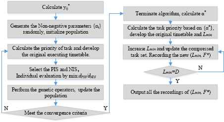
A flowchart of the solution procedure.
3.3.2 Reactive Allocating for Type 2 Design Change
In this paper, we consider the complete compression for one arrival task which means that all the compression is applied to the arrival task only. If an uncertain task arrives at VDU i, we use some (possibly extraordinary) mechanism (such as overtime) to get the allocation back on track by reducing the task executing times at an additional cost of cj^ per unit of executing time reduction for task j^. The compression costs in this condition is a linear function of compression time ej^ – τj^. In such cases,
Expressing the expected cost zq_i (t) as a function of z(q_i)–1 (t), we have that zq_i (t) equals z(q-i)–1 (t) added to the expected compression cost, and the unused idle time cost of the task j^, which we express using the function
Based on our prior construction and discussion, zq_i(t) provides the minimum cost of the scheduling job task [q_i] with an expected finish time of t. Note that the value of zq_i (t) for some [q_i] and t combination may be infinite, which implies that no feasible schedule exists for job [q_i] finishing at time t. The optimal value of the objective function for the fixed sequence is then given by
We next characterize the complexity of the dynamic programming approach. Let ρmax denote the largest executing time compression possible among all tasks. In the recursive equation of compression cost, if t′ > r[q_i], then for each t, there are O(ρmax) possible values of τ[q_i], and one value of t′ for each [q_i]. Therefore, z(q_i)–1 (t′) is determined for each τ[q_i]; if t′ ≤ r[q_i], then for each t, there is one value of τ[q_i], and we select the t′ that gives the lowest value of z(q_i)–1 (t′). Given a (q_i, t) pair (a state), we require O(ρmax) operations to compute Formula (13). In each stage (task) there are O(ρmax) states. Selecting the lowest value of z(q_i)−1 (t′) requires O(ρmax) operations for each stage. Therefore, we need
In this section, we consider the Compression to absorb the disruptions, as we show next. This problem is equivalent to a deterministic scheduling problem with controllable processing times.
We assume that all the time variables and parameters are integral multiples of a proper unit of l. As before, our predictive policy schedules τ[
q_i] units of planned idle time, where
Given a predictive schedule, the expected cost and the objective function will be as follows:
Note that the
4. Computational Study
4.1 Reactive Allocating
In this paper, we use the random numerical test to verify the effectiveness of this method. In task assignment problem fields, we use the conventional method to solve this problem. Specific design task attributes, design capability attributes of VDU, task classification criteria, and other information are described in the research of Cao et al.43. The literature has considered the sorting problem in the case of VDUs that are not available at some point. Some scholars have taken the stochastic arrival of tasks into account and asked for emergency processing.
The problem has been proved to be an NP-hard problem and the SPT rule can minimize the expected time when the VDU unavailability is the exponential distribution. Therefore, the use of SPT to form the initial executing timetable is a better way to deal with the possible interference events. In this part, we assume that the losing time Xi of VDU i and the recovery time Yi are subject to the exponential distribution of the different parameters respectively. In the following, PDS stands for our proposed probability distribution sequencing, so that SPT stands for the shortest processing time method. A comparative analysis of the original allocating timetable of PDS and SPT is performed in this section.
We let the size be n =100, m = 5 and n = 200, m = 6, respectively. For the practicality of the verification method for the general situation, the residual parameters are randomly generated from a uniform distribution. We generated the design cost for each task-VDU pair randomly from Uniform [2.0,6.0]. For the compression function, the coefficient h is randomly generated from the interval [1.0,3.0]; aij/bij is randomly generated from the interval [1.1,3.1]. For the executing time,
For PIS and NIS, let PIS be (0,0) and NIS be a two-dimensional vector consisting of the minimum match-time point and the corresponding compression cost in the original allocating timetable generated by SPT. The GA in Figure 1 is achieved by MATLAB 7.6.0.324. The population is grouped by continuous real number coding and the population size is 15. The initial population is randomly generated. The calibration function uses the Rank function to map the target function values of the individual to the position in the objective function value. This method can avoid fluctuations in the original target value. The selection operations are based on a random stochastic uniform function, the cross operation is a scattered cross, and the mutation operation is based on a Gaussian function. The parameters in the genetic operation are the default values.
When it generates individual offspring, the number of elite individuals is 2. The next generation of individuals from the cross product is 80%, the mutation product is 20%. The maximum evolutionary generation is used to control the output of the genetic algorithm with the set of the maximum evolutionary generation equal to 100. The remaining parameter settings are all the default values. For each combination of n – m – β, we repeat 15 calculations. Each calculation generates an example randomly. Comparing the original allocating timetable of SPT and PDS to estimate the result interval. For n = 100, m = 5, β = 0.10, and Pd(t) is shown in Figure 2.
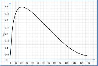
The production design cycle.
From Figure 2, we can see that the maximum value of Pd(t) is obtained in the product design cycle. Corresponding to the parameters in Figure 2, the comparison of the original executing timetable is based on PDS and SPT, respectively, as shown in Figure 3.
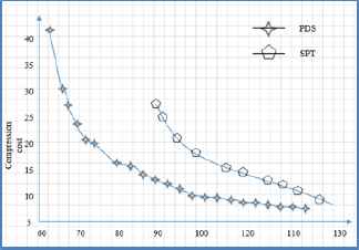
The typical computing result.
From Figure 3, it is obvious that there is an offsetting-restricting relationship between the match-up time point and the compression cost. With the increase of the match-up time point, the compression cost will decrease. The greater the match-up time point, the greater the impact caused by the design change. When the match-up time point increases to the maximum completion time of the task, the compression cost is minimum. However, all the tasks have been affected by the design change at its worst case which is unacceptable in our design environment especially.
As can be seen from Figure 3, the minimum match-up time obtained by PDS is 62.45, which is better than 88.98 obtained by SPT. The compression cost of PDS is lower than SPT when the minimum match-up time is 88.98 obtained by SPT. When the match-up time is equal to Di, the compression cost of the two methods is relatively close, the cost of PDS is slightly lower.
In order to further quantify the effectiveness of our approach, several indexes are used to measure the results of multiple experiments and the PDS is compared with the SPT. The indicators involved and their meanings are describedas follows.
The number (NUM) of match-up time points is selected by the decision maker. For SPT, it is the number of two-dimensional vectors (Lmin, F*) that are finally output by the algorithm flow shown in Figure 1. For SPT, similar to the flowchart in Figure 1, after obtaining the minimum match-up time point, we increased the point successively when the corresponding compression cost is calculated until the match-up time point is equal to the length of the original allocating timetable. In short, the greater the number is, the more the room for decision-makers to choose.
The minimum match-up time (MMT) and the average match-up time (AMT) are the optimal value and the mean value of the match-up time points, respectively, which is the core point that the decision maker should pay attention to in the design process. The bigger the point is, the more external activities that depend on the original allocating timetable, such as resource configuration, the next processing arrangement of the task, and so on.
The cost at the same time (CAT) indicates the respective compression cost of the PDS and SPT at the minimum match-up time point obtained by SPT. This indicator considers the problem from the point of view of comparing the cost of different methods at the same match-up time point.
The Minimum cost (MC) and the Average cost (AC) correspond to the MMT and AMT and reflect the increasing minimum cost and the average cost to restore to the original allocating timetable.
Robustness is an emphasized objective so that it recovers to the original allocating timetable and is required after the occurrence of the design change. Therefore, MMT and AMT are of the utmost importance of the above indicators.
Table 1 shows the average value of 15 tests for each parameter combination. Table 2 provides an interval estimate of the average improvement rate for the 15 tests with respect to SPT in terms of the number, MMT, AMT, and so on.
| Index | Type | Method | n = 100, m = 3, β | n = 200, m = 6, β | ||||||
|---|---|---|---|---|---|---|---|---|---|---|
| 0.10 | 0.12 | 0.13 | 0.15 | 0.10 | 0.12 | 0.13 | 0.15 | |||
| NUM | max | PDS | 32.73 | 29.87 | 28.33 | 25.33 | 65.00 | 61.07 | 57.47 | 41.07 |
| SPT | 11.07 | 8.47 | 7.73 | 6.33 | 18.80 | 16.73 | 13.67 | 11.60 | ||
| MMT | min | PDS | 65.20 | 65.76 | 75.39 | 79.95 | 124.31 | 132.97 | 139.97 | 168.28 |
| SPT | 92.70 | 95.16 | 100.31 | 100.90 | 184.69 | 194.04 | 199.44 | 207.78 | ||
| AMT | min | PDS | 92.45 | 90.67 | 97.47 | 98.23 | 178.21 | 184.98 | 187.42 | 203.31 |
| SPT | 106.79 | 106.01 | 110.23 | 108.90 | 208.91 | 216.50 | 218.28 | 223.72 | ||
| CAT | min | PDS | 18.2 | 24.84 | 28.41 | 37.39 | 28.28 | 45.99 | 46.31 | 69.36 |
| SPT | 29.97 | 32.64 | 46.44 | 54.88 | 51.39 | 75.52 | 82.49 | 103.72 | ||
| MC | min | PDS | 26.03 | 40.15 | 36.64 | 46.76 | 42.59 | 71.73 | 70.28 | 86.25 |
| SPT | 16.48 | 20.83 | 30.07 | 38.85 | 29.07 | 43.94 | 51.55 | 70.49 | ||
| AC | min | PDS | 10.52 | 15.85 | 21.14 | 31.40 | 17.32 | 28.46 | 32.22 | 53.44 |
| SPT | 9.75 | 14.14 | 20.64 | 28.83 | 17.54 | 28.44 | 35.19 | 51.52 | ||
A comparison of the absolute metric values of PDS and SPT.
| n | Index | β = 0.10 | β = 0.12 | β = 0.13 | β = 0.15 | ||||
|---|---|---|---|---|---|---|---|---|---|
| Lower | Upper | Lower | Upper | Lower | Upper | Lower | Upper | ||
| 100 | NUM | 1.61 | 2.68 | 2.11 | 3.52 | 1.87 | 3.60 | 2.15 | 3.93 |
| MMT | − 0.33 |
− 0.26 |
− 0.33 |
− 0.28 |
− 0.32 |
− 0.18 |
− 0.27 |
− 0.14 |
|
| AMT | − 0.15 |
− 0.12 |
− 0.16 |
− 0.13 |
− 0.15 |
− 0.08 |
− 0.13 |
− 0.07 |
|
| CAT | − 0.47 |
− 0.29 |
− 0.35 |
− 0.07 |
− 0.47 |
− 0.25 |
− 0.39 |
− 0.25 |
|
| 200 | NUM | 2.23 | 2.78 | 2.39 | 3.05 | 2.81 | 3.95 | 1.89 | 3.20 |
| MMT | − 0.34 |
− 0.31 |
− 0.33 |
− 0.29 |
− 0.31 |
− 0.29 |
− 0.24 |
− 0.14 |
|
| AMT | − 0.15 |
− 0.14 |
− 0.16 |
− 0.13 |
− 0.15 |
− 0.13 |
− 0.11 |
− 0.07 |
|
| CAT | − 0.51 |
− 0.38 |
− 0.43 |
− 0.33 |
− 0.47 |
− 0.40 |
− 0.39 |
− 0.23 |
|
The 95% CI estimates of the improvement on the critical metrics of our method.
Data in Table 1 and Table 2 retain two decimal places. In this paper, a confidence level of 95% is used to estimate the confidence interval. For a certain index, the improvement rate is calculated as follows.
In addition, MMT and AMT of PDS are smaller than the corresponding items of SPT, indicating that the original allocating timetable given in this section is subject to interference events during the executing phase and can restore the system plan as early as possible. This can effectively reduce the impact of design change. Although AC of PDS is higher, the earlier match-up time points in the design process can reduce the larger losses caused by the design change. Finally, the same cost indicator in the vicinity of the MMT shows that the compression cost of PDS is lower than SPT. In this paper, PDS can significantly reduce the match-up time after the occurrence of the design change and improve the selectable range of the decision, and the compression cost can be significantly reduced by SPT in the vicinity of the MMT. Therefore, PDS gives priority to the compression time while taking the compression costs into account.
In summary, PDS constitutes an original allocating timetable relative to SPT, which can be more effective in coping with the design cost, and the design system can be restored to the original plan as soon as possible.
4.2 Reactive Allocating
It is worth mentioning that the size of experiment and some parameters have been determined by the proposed method based on data verification. To simplify this problem, the inserting idle time is based on the sequence has been identified by PDS.
Table 3 summarizes the experimental conditions. β = 0.12 shows its advantage in section 4.1. Therefore, β = 0.12 is chosen as a fixed parameter in the exponential distribution of random unavailability. The new tasks are assigned to VDUs according to their attributes of design capacity, and then the position and the idle time for the new tasks are determined within their probability distribution.
| Dimension | Characteristic | Specification |
|---|---|---|
| Size | n = 200, m = 6, β = 0.12 | |
| CPD process | Tasks arrival rate The number of new tasks Task release policy Random arrival Random unavailability Executing time of a design task |
[0.125, 0.25, 0.5, 1] [10, 20, 40, 60, 80, 100] Immediate Passion distribution Exponential distribution [1, 10] |
| Performance measures | Makespan Stability Robustness Compression cost |
|
The experimental conditions.
The most popular predictive approach in the project management and machine scheduling literature is to leave the idle times (time buffers) in schedules in coping with disruptions. The quality of the proposed method PDS+IIT is compared with the SM(τ) reference of Yang and Geunes26.
PDS+IIT+ CETS: here, we generate the predictive allocation by the proposed PDS +IIT, CETS as the reactive policy.
The SPT+SM(τ)+CETS: SPT + SM(τ) policy is used to generate the predictive allocation, CETS is for the reactive policy.
The SM(τ) policy is used to generate an effective allocation to provide a good solution using the SM method (SM is a basic and effective heuristic method developed by Rachamadugu and Morton44), and then τ units of idle time for the tasks are inserted at some point in the allocation (both the amount of planned idle time and the insertion position are decision variables), where τ is integer.
Table 4 and Table 5 show the performance comparison between the proposed method PDS +IIT+ CETS and the other method SPD+SM(τ)+CETS. β = 0.12 is a fixed index in the exponential distribution of the unavailability of VDU. Therefore, the computational experiments are performed to compare the two methods. A quantity of six new task arrivals (10, 20, 40, 60, 80, 100) forms the first factor. It is grouped into three types of new task arrivals (small: 10, 20; medium: 40, 60; and large: 80, 100). Two task arrivals are rated λ; namely, the sparse and dense task arrivals are considered (sparse: 0.125, 0.25; dense: 0.5, 1).
| Policy/performance | PDS +IIT+ CETS | SPD+SM(τ)+CETS | |||||||||
|---|---|---|---|---|---|---|---|---|---|---|---|
| λ/Scale | Ma. | St. | Ru. | Co. | Ma. | St. | Ru. | Co. | |||
| λ | 0.125 | S | 10 | 156.23 | 47.23 | 102.44 | 23.44 | 174.63 | 53.63 | 102.44 | 33.65 |
| 20 | 171.44 | 55.20 | 113.36 | 26.58 | 188.36 | 64.38 | 113.36 | 39.59 | |||
| M | 40 | 195.26 | 60.58 | 126.32 | 29.36 | 214.63 | 71.26 | 132.25 | 42.36 | ||
| 60 | 213.32 | 71.15 | 134.55 | 33.56 | 245.29 | 80.65 | 142.85 | 48.56 | |||
| L | 80 | 241.85 | 84.62 | 145.36 | 39.64 | 266.86 | 86.59 | 151.36 | 52.57 | ||
| 100 | 263.16 | 92.37 | 156.39 | 49.63 | 285.64 | 98.47 | 163.25 | 56.93 | |||
| 0.25 | S | 10 | 164.54 | 52.36 | 109.52 | 34.26 | 186.78 | 60.12 | 109.52 | 36.85 | |
| 20 | 181.23 | 59.38 | 116.32 | 41.28 | 204.63 | 69.25 | 116.32 | 44.56 | |||
| M | 40 | 214.59 | 68.94 | 125.68 | 49.29 | 224.69 | 71.36 | 125.68 | 51.96 | ||
| 60 | 245.93 | 79.53 | 133.27 | 54.31 | 259.36 | 86.34 | 139.56 | 58.39 | |||
| L | 80 | 266.51 | 89.64 | 145.69 | 61.88 | 286.61 | 94.28 | 159.98 | 69.65 | ||
| 100 | 287.75 | 104.35 | 163.52 | 71.36 | 298.64 | 109.88 | 170.25 | 74.44 | |||
The performance measures of the two methods with sparse task arrivals.
| Policy/performance | PDS +IIT+CETS | SPD+SM(τ)+CETS | |||||||||
|---|---|---|---|---|---|---|---|---|---|---|---|
| λ/Scale | Ma. | St. | Ru. | Co. | Ma. | St. | Ru. | Co. | |||
| λ | 0.5 | S | 10 | 165.59 | 47.23 | 102.44 | 29.36 | 187.36 | 55.36 | 102.44 | 35.62 |
| 20 | 178.86 | 55.20 | 113.36 | 34.89 | 196.36 | 69.14 | 116.32 | 42.58 | |||
| M | 40 | 201.85 | 60.58 | 135.25 | 46.52 | 209.36 | 72.36 | 142.36 | 49.62 | ||
| 60 | 211.96 | 76.15 | 146.93 | 57.65 | 230.86 | 81.36 | 153.96 | 56.32 | |||
| L | 80 | 218.74 | 94.62 | 156.39 | 68.22 | 252.54 | 91.20 | 164.85 | 64.21 | ||
| 100 | 223.61 | 106.37 | 166.84 | 78.12 | 271.95 | 100.92 | 171.94 | 75.25 | |||
| 1 | S | 10 | 192.54 | 52.36 | 109.52 | 34.98 | 195.36 | 58.56 | 109.52 | 38.65 | |
| 20 | 224.82 | 70.38 | 116.32 | 46.10 | 230.36 | 72.85 | 121.63 | 44.21 | |||
| M | 40 | 251.76 | 81.94 | 146.85 | 57.74 | 259.36 | 80.64 | 155.93 | 57.21 | ||
| 60 | 276.16 | 95.53 | 153.85 | 65.66 | 281.69 | 93.85 | 163.86 | 63.21 | |||
| L | 80 | 283.39 | 107.64 | 162.55 | 77.33 | 293.53 | 101.22 | 171.22 | 74.64 | ||
| 100 | 301.58 | 116.35 | 176.89 | 86.96 | 310.26 | 108.34 | 186.57 | 84.12 | |||
Ma. : Makespan; St. : Stability (deviation); Ru. : Rubust (Minimum Match-up time); Co. : Compression cost
The performance measures of the two methods with dense task arrivals.
The results in Table 4 and 5 indicate that the proposed method PDS +IIT+CETS outperforms SPD+SM(τ)+CETS from the four measures in most experimental data. It is more capable of achieving the optimal solutions for most case studies. In the experiment with sparse task arrivals, the proposed method PDS +IIT+CETS performs with the absolute advantage on all of the measures.
When the reactive conditions are more complex (the value setting of the task arrival rate and the quantity of new tasks becomes bigger), a reversal appears in some performance. This is obvious in the experiments with dense task arrivals. When the value of λ is equal to 1, the quantity is greater than 20, the stability and compression cost of SPT+SM(τ)+CETS are greater than PDS +IIT+CETS. This indicates that once there exists a more complicated disruption, a predictive inserting idle time method for all the tasks is a more effective way than the proposed method. Minimizing the insertion of the idle time is an effective method to improve the resource utilization with sparse task arrivals. However, in the condition of dense task arrivals, it becomes more difficult to control the compression cost and the stability.
The results also indicate that the proposed method performs well for different parameter settings. It can be observed from the table that it requires more compression time to absorb the disruptions as the number of tasks increase. As expected, as the length of the disruption is increased, the proposed method tends to generate a better solution for the match-up time problem.
In this section, we have shown that we can efficiently solve match-up rescheduling problems with a controllable executing time exactly by using recently developed reformulation techniques and commercial solvers. It is observed that the heuristic algorithm is able to generate a good approximation of the efficient frontier of match-up time and compression cost quickly. When the quantity of new tasks is consistent, the influence on allocation is positively associated with the arrival rate. Similarly, when the quantity is given, the influence is positively associated with the arrival rate as well. The ambiguity in the description of the coordination cost and the different measurements are the main influencing factors for decision-makers. In the real-world design process, the objectives for practitioners are different. Some concentrate on the design cost, some focus on time, and some think of the stability, robustness, or even the balance between them. Therefore, the four performances provide a reference for decision-makers to make a scientific and rational decision considering their individual situation.
5. Conclusions
In this paper, a robust predictive–reactive allocating approach is proposed with controllable executing times. The design change is considered in preparation for the original predictive allocation with anticipative probability distributions. We showed that the predictive decision making in preparing original allocations can avoid excessive reallocating costs resulted by reactive executing time adjustments and this ensured the strong robustness and stability of the design system.
In the phase of predictive allocating, the probability of the design change is utilized to generate the combinatorial approach with PDS and IIT. In PDS, we estimate which task can absorb a possible interference with the lowest cost, then determine the task sequence on each VDU. Based on sequence, the IIT policy is used to respond to task arrivals. This effective combination of PDS and IIT can absorb almost all of the interference impact caused by the design change. Four measurements, which are Cmax, stability, robustness, and compression cost, are adopted in this paper to mirror the quality of the proposed approach. The application of combinatorial optimization is tested and verified by a computational simulation. The results of comparing two methods within the different setting of the parameters show its effectiveness. Two factors, which are the task arrival rate and the quantity of the task arrival, and their interactions are analyzed in section 4 to indicate the interference impact caused by the design change.
While the findings of this study improve our understanding of the task allocations in the complex product design process, its limitations should also be recognized. First, in this paper, we suppose that the design change obeys some certain distributions. However, in the real design process, the appearance of design change is more complex and difficult to predict. Second, the scale and complexity of the hypothetical design change in this paper are not fully considered. Lastly, the compressing character in this paper assumes that all the execution objects accept this adjustment and act in concert with other departments. The situation that some execution objects may not want to change their work is also not our research focus.
Therefore, in order to further improve our research, further research would be definitely called for. First, as this paper only consider the exponential distribution for VDU unavailability, it may be interesting to consider the different combination of Normal-Normal, Triangular-Normal, Exponential-Normal, Exponential-Exponential distributions, and so on. Second, it will be interesting to consider the scale and complexity of the design change to improve the accuracy of the predictive phase. Finally, in the further research, the different changing will of the execution objects should be considered to better reflect the design process and enhance the quality of the findings.
Acknowledgements
This work is supported by the National Science Foundation of China (71701027), the Open Funding of Chongqing Technology and Business University (KFJJ2017082), China Postdoctoral Science Foundation funded project (2016M590929), and the Humanity and Social Science Youth Foundation of Ministry of Education of China (IZYJC630198).
References
Cite this article
TY  - JOUR
AU  - Jiafu Su
AU  - Meng Wei
AU  - Aijun Liu*
PY  - 2018
DA  - 2018/07/12
TI  - A Robust Predictive–Reactive Allocating Approach, Considering Random Design Change in Complex Product Design Processes
JO  - International Journal of Computational Intelligence Systems
SP  - 1210
EP  - 1228
VL  - 11
IS  - 1
SN  - 1875-6883
UR  - https://doi.org/10.2991/ijcis.11.1.91
DO  - 10.2991/ijcis.11.1.91
ID  - Su2018
ER  -