
Salary Prediction in the IT Job Market with Few High-Dimensional Samples: A Spanish Case Study
- DOI
- 10.2991/ijcis.11.1.90How to use a DOI?
- Keywords
- Salary prediction; e-Recruitment; Job Market; Machine Learning; Ensemble methods
- Abstract
The explosion of the Internet has deeply affected the labour market. Identifying most rewarded and demanded items in job offers is key for recruiters and candidates. This work analyses 4, 000 job offers from a Spanish IT recruitment portal. We conclude that (1) experience is more rewarded than education, (2) we identify five profile clusters based on required skills and (3) we develop an accurate salary-range classifier by using tree-based ensembles.
- Copyright
- © 2018, the Authors. Published by Atlantis Press.
- Open Access
- This is an open access article under the CC BY-NC license (http://creativecommons.org/licences/by-nc/4.0/).
1. Introduction
Accurate recruitment of employees is a key element in the business strategy of every company due to its impact on companies’ productivity and competitiveness. At present, recruitment processes have evolved into complex tasks involving rigorous evaluations and interviews of candidates, with the goal of hiring the best suited professionals for each company’s needs. With the advent of Internet and the web, e-Recruitment has become an essential element of all hiring strategies. Many websites, such as Career-Builder, Monster or Tecnoempleo, or even Social Networks, like LinkedIn, help companies and job seekers to find the best possible matches.
e-Recruitment is a very active topic of research and its impact in the industry has been addressed by several studies (see Refs. 1–6). On the recruiter side, recent applications include: a framework for candidate ranking and résumé summarization to improve recruiter’s performance (Ref. 7), a novel tool for candidate evaluation that adapts to the feedback received (Ref. 8), a tool for automatically evaluating candidates’ CVs (Ref. 9), and a system to screen candidates and score them, thus enabling candidate filtering and reducing the workload of recruitment officers (Ref. 10). In the area of job recommendation, several systems have been proposed which recommend jobs according to candidate profiles obtained by clustering techniques (see Refs. 11–15).
Machine learning methods have also been extensively applied to e-Recruitment. In Ref. 16, the authors propose a machine learning model for detecting talent and updating company’s knowledge taxonomy, which helps recruiters to detect and incorporate the professional profiles the company lacks. In Ref. 17 the authors employ different classification and clustering techniques and in Ref. 18 the authors automatically group job offers using supervised machine learning combined with expert labelling. Promising results have been shown also in Ref. 19, where the authors revert to pattern recognition in order to predict competency or skill emergence in the job market. Some studies have also proposed systems and databases enriched by data mined from the web (see Refs. 20, 21). In particular, the use of social networks for recruitment purposes has gained attention recently, specially on the recruiter side. For example, in Ref. 22 an expert retrieval system is presented based on profile information and user behavior inside different social networks (Twitter, Facebook and LinkedIn). In Ref. 23 an expert-finding algorithm is proposed based on location and connections to potential candidates.
Most of the works that focus on the extraction of insights from e-Recruitment portals retrieve the information associated with each job post as text and then they represent each sample as a vector of word/keyword frequencies. As a consequence, these vectors are often characterized by a very high number of dimensions (in the order of thousands). Therefore, it is necessary to collect huge amounts of job posts to be able to train a classifier or a regression model effectively. However, for websites with a limited target audience, such as portals developed for a specific geographic area or job sector, there are relatively few job posts. Among these, only a small percentage has an explicit indication of the offered salary. This can make the prediction of the salary from the job post features a challenging task.
In this work we present a case study based on data collected from an e-Recruitment website specifically designed for IT jobs in Spain, named Tecnoempleo†. The website contains a large collection of job offers, containing many machine-readable fields which are not common in other similar sites, such as the requested skills. However, only a small portion of posts include the offered salary. As a result, our dataset, which covers a period of 5 months, includes only ≈ 4,000 job posts, which are represented as vectors of ≈ 2,000 features. In this context characterized by data scarcity and high dimensionality, we extract useful insights from the data and employ an ad-hoc feature engineering procedure to mitigate the effect of noise and increase the accuracy of salary prediction.
In more detail, the main contributions of this paper are:
- •
the proposal of a manual feature preprocessing to clean, format and standardize the collected data, and to reduce dimensionality by 10 times while improving the prediction accuracy, with no need of any other automatic feature selection procedure;
- •
an investigation on which fields in a job post have greater influence on salary and how they are interrelated;
- •
the discovery of the main data-driven profiles obtained through skill-set based aggregation;
- •
the formulation of the salary prediction problem as a classification task in order to have a better accuracy by focusing on discrete ranges instead of continuous salary values;
- •
the comparison of several classifiers, including SVM, MLP, random forests, AdaBoost and ensembles of them, in order to find the model with the best accuracy in predicting the salary range. This model can be effectively employed by an e-Recruitment website to provide an automatic categorization of job posts by salary range, even when the real offered salary is missing, or used as a building block in a job recommender system.
The reminder of this work is structured as follows: Section 2 describes the most relevant algorithms and methods used as well as the data gathering and feature engineering processes. Section 3 reports the descriptive analysis performed to understand the data and obtain interesting insights and data-driven job profiles. Then, Section 4 presents our detailed classifier comparison and Section 5 reviews the results.
2. Methodology
The dataset under study comprises 3,970 job posts. In order to gain useful insights into the online job recruitment for IT professionals, we compare and contrast different strategies and machine learning models. The methodology follows the best practices in the literature and in the industry, including different phases:
- 1.
Data collection: a Python-based web crawler‡ is developed to parse and gather the necessary information from the website. The crawler was run on a daily basis from December 2015 to April 2016 and duplicates were removed.
- 2.
Data cleaning: posts with missing values are removed and possible conflicts in the data format (e.g. text encoding) are fixed.
- 3.
Manual feature engineering: irrelevant features are discarded and others are standardized (e.g. converted into numerical features) by exploiting the domain knowledge.
- 4.
Dataset description: statistical tools and simple models are used in order to provide a preliminary and compact description of the data.
- 5.
Automatic feature selection: feature selection algorithms are employed to automatically select the most informative features in the dataset with respect to the output class.
- 6.
Model selection: a grid search is performed to find the optimal hyper-parameters for a set of well-known machine learning models.
- 7.
Model training and validation: the selected models are trained and cross-validated in order to find the classifiers that best describe the data and are able to predict the output variable with the highest scores.
- 8.
Model comparison: each model is compared to the others with respect to standard scores and curves like the classification accuracy, the F1 score, the ROC curve, the Precision-Recall curve etc.
The raw data collected by using the crawler are not useful without an accurate preprocessing phase to remove the sources of noise and normalize the remaining data. In addition, one also has to decide how the missing values should be treated. In this case, samples with missing values were removed because in most cases they cannot be substituted by any default value.
Unstructured information like the title of the job post as well as the textual description of the requested profile and the offered position was also removed. Among the technology keywords that describe each post, we noticed that some of them consist only of numbers, probably related to the versions of the software required by the companies. These are clearly not useful for the salary prediction.
Since most of the keywords are manually introduced by users, it is also essential to unify the data format by merging semantically equivalent words, their different translations (e.g. in English or Spanish) and typographic errors. For example, keywords like administracion, adm, administrativo, administration should appear in the dataset as a unique feature: administration. Part of this process might be automated by using dictionaries, but it becomes more difficult for error correction. A way to improve the categorization of the different job posts on the web portal is to give the user the possibility to choose only from a predefined set of keywords. In this way one also prevents the sparsity of the keywords.
In our work, we do not consider all the keywords that appear less than 10 times (corresponding to 0.25% of the total number of job posts). This results in the removal of hundreds of features that can be considered as noise.
We also remove posts for jobs not located in Spain. By removing missing values, noisy features and unstructured data, it was possible to reduce the number of features to ≈ 200 (from ≈ 2,000 in the raw dataset as collected by the crawler).
An important role in the feature preprocessing has also been given to the translation of categorical features into numerical features. In summary, the dataset is modified as follows:
- •
the feature describing the dedication (full-time, part-time or autonomous work) is transformed into the maximum number of week hours: 40 for full-time jobs and 20 for part-time and autonomous jobs. Autonomous jobs are considered equivalent to part-time jobs because most of the times they refer to limited periods of time;
- •
the feature that describes the incentives offered by a company is substituted by a boolean feature that indicates the presence or absence of incentives;
- •
the minimum education level (described by words) is converted to the minimum number of education years according to the Spanish education system. All the levels that do not fall in the main categories as listed on the website are assigned the same number of years of compulsory education (10 years, age 16). For the other values, see Table 1;
- •
for each of the 488 companies that posted a job offer, we retrieve the approximate number of employees. This is used as an indicator of the company size, which can be related to the number and frequency of job posts. For most of them we retrieve the information from their public social profiles (e.g. LinkedIn). In case this information is not publicly available, the information is completed with the median value of workers in the rest of the companies;
- •
the textual representation of working experience is translated into the average number of years. For example, 2years is substituted by 2, while 3–5years by 4;
- •
we describe the type of contract by using 3 mutually-exclusive binary features (represented with the so-called one-hot encoding), which indicate whether a job post is related to a permanent, temporary or other type of position (e.g. a hourly service);
- •
we introduce the per capita gross product in the geographic region of each company. This is reasonable if one considers that the highest salaries are usually clustered around the most important economic centers.
We also rescale all features to the interval [0,1] by normalization on the range given by the maximum and minimum values of each feature.
| Education level | Min. years in education |
|---|---|
| School | 10 |
| High School | 12 |
| Professional formation (PF) | 12 |
| Higher PF | 14 |
| Engineer | 15 |
| Graduate (Bologne) | 15 |
| short Degree | 15 |
| Engineer | 17 |
| Degree | 17 |
| Msc. (Bologne) | 17 |
| PhD | 20 |
Correspondence between education levels and minimum number of years in the education system for Spain.
To derive useful insights from the data, we employ regression models and clustering algorithms based on the numerical feature salary as obtained by the crawler (see Section 3). These algorithms include:
- •
K-means clustering, which is useful to partition the data in homogeneous groups (see Ref. 24 for a description of the basic concepts);
- •
Linear Regression, which models the relationships between the features and the output variable as linear functions;
- •
Regularized Linear Regression, which introduces a penalty into the error function dependent on the feature weights to avoid overfitting and to automatically select the most relevant features.
Two well-known regularization methods are based on ℓ1 and ℓ2 norms (see Refs. 25, 26). These models are often used as the baseline in several contexts and sometimes are sufficient for a highly accurate prediction (see Refs. 27, 28).
In order to quantify the performance of a linear model, we consider the coefficient of determination (R2), which provides an assessment of the variability of the output any linear model is able to capture and depends on the variance of the data and the sum of the squared errors of the model.
Despite the usefulness and simplicity of the previous approaches in describing the data, our main focus is on the prediction of salary ranges, because this can result in a better categorization of the job posts and thus an easier navigation for the end-users. This is also motivated by the specific case study we are addressing, that is, predicting the salary associated with a job post, when the number of posts with an explicit indication of salary is low. In this context, the prediction of discrete ranges should be more accurate than the prediction of the actual salary, which is a continuous number. To accomplish this, each job post is assigned to one of four classes, which represent salaries in the low, medium-low, medium-high and high ranges. These ranges are decided according to the values of the first, second and third quartiles (also known as Q1, Q2, and Q3).
After formulating the prediction problem as a classification task, we compare different models for finding the classifier that best explains the data in a job recruiting scenario characterized by high level of noise, high dimensionality and a limited set of samples. We consider several solutions based on:
- •
Linear models (LM);
- •
Logistic regression (LR);
- •
K-nearest neighbors (KNN);
- •
Multi-layer perceptrons (MLP);
- •
Support vector machines (SVM);
- •
Random forests (RF);
- •
Adaptive boosting with decision trees (AB);
- •
Ensembles of the previous models.
Recent applications of LM, LR, KNN, MLP and SVM are Refs. 29–36.
In most real-world scenarios, there is no clear winner among several individual classifiers and most of the times combining two or more models into a committee or an ensemble is beneficial with respect to the classification performance of the overall system. Examples are random forests (RF), which employ a set of decision trees trained on random subsets of the original data, and boosting algorithms, which are iteratively built upon one simple model that is progressively improved (or boosted) by penalizing samples misclassified in the previous iteration. Recent applications of RF and boosting algorithms, in particular the well-known Adaptive Boosting algorithm (AdaBoost or AB) can be found in Refs. 37–40.
Other approaches for ensemble learning are possible such as voting classifiers. In this case a committee of n heterogeneous weak models is trained so as to have n independent predictions of the class of a sample. The final decision on the output variable is then the result of a majority vote among the members of the committee. In our work we use two variants of a voting classifier: one that includes all the other classifiers that we compare in the tests (Vote), and one that includes only the top-3 best performing models (Vote3). Other examples of ensembles are presented in Refs. 41–47.
Concerning automatic feature selection, we use the filter method X-MIFS (see Ref. 48), which is one of the state-of-the-art algorithms for selecting features based on the maximization of the mutual information (MI) between the features and the output variable. This technique is based on a generalization of the MI to multiple features. In particular it evaluates the MI between the whole set of selected features and the class, so as to add only those features that are relevant when considered together. We decided to use a filter method, as opposed to wrapper and embedded methods, because of its scalability to high-dimensional data and independence from the classifiers used. In addition, the MI measures arbitrary dependencies between random variables, and it is suitable for assessing the information content of features in complex classification tasks. Moreover, the MI metric does not depend on the particular machine learning model or choice of coordinates. We included this automatic feature selection method to test for the existence of an optimal subset of features that can improve the accuracy but would be difficult to extract during the manual preprocessing.
In our experiments we also used a preliminary deterministic grid search on all the parameters involved within specific ranges of values. The final tests were conducted by using, for each family of classifiers, the configuration that gave the best average classification accuracy in a 3-fold cross validation. The scores used for comparing the different algorithms include:
- •
the classification accuracy, which is the percentage of correctly classified samples;
- •
the precision, which is defined, for one specific class, as the fraction of true positives among the samples predicted to belong to that class (true and false positives);
- •
the recall, which is defined, for one specific class, as the fraction of true positives among the samples belonging to that class (true positives and false negatives);
- •
the F1 score, which is the harmonic mean of precision and recall;
- •
the area under the precision-recall curve (AUCPR) built for different thresholds of the probability of the positive class;
- •
the area under the ROC curve (AUC-ROC) that shows the true positive rate against the false positive rate for different thresholds of the probability of the positive class.
For all the class-specific scores, we compute the average on all the classes in order to obtain a scalar value for each model.
Before looking at the experimental results on the classifier comparison, in the next Section we describe the dataset in more detail by using some descriptive statistics, a simple linear regression model for job salary prediction and two job clustering experiments looking for groups of job posts in terms of either salary or demanded skills. In this way it is possible to better understand the data with some insights that can be useful to explain the results of Section 4.
3. Dataset inspection
Job posts in our collection are related to 488 companies with an average number of offers per company of 8.13. However, Fig. 1 shows that the distribution of job posts is heavy tailed, with most companies (exactly 71.7%) posting only one or two job offers. For visualization purposes, the x-axis, which depicts the number of offers per company is scaled to the base 2 logarithm, so different buckets (bars) contain an incremental number of offers (e.g. the first bucket includes companies with one or two job postings, the second bucket includes those offering 3 or 4, and the last bucket includes all companies offering between 512 and 1024 job postings).
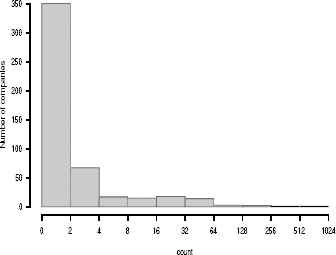
Number of companies against the number of job posts (log-scale).
As an example, Company 353 (company names have been anonymized for privacy reasons), which is the most active, posted a total of 681 job offers, and only six other companies posted more than 100 offers.
Similarly, the geographical distribution of posts is not uniform, being more frequent in cities, in particular the biggest cities in Spain. Fig. 2 displays the number of posts in a map§, thus showing that Madrid and Barcelona accumulate more than 80% of the total positions while the rest is still unevenly distributed between regional capitals and other cities. These cities are the largest in Spain in terms of population and have the highest pro-capite income.
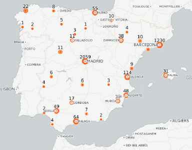
Geographical distribution of job posts.
Among the features of each post, Job Position specifies what is the role to be covered by any applying candidate. Fig. 3 shows a set of the most frequent job positions (and their frequencies), with the most demanded position being Programmer, followed by Administrator and Technical Support. Interestingly, Programmer positions are required in more than half of the available posts, thus suggesting a clear demand of highly technical profiles.
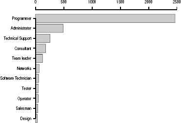
Most frequent job positions.
As expected, the most demanded skills are mainly IT and technological skills. For instance, technologies such as .Net or Java appear in 16.9% and 16.7% of job posts respectively. Others like SQL (11.7%), Javascript (9.3%) or PHP (8.8%) are also highly demanded.
Other relevant features are experience and education. The average required experience is 2.45 years, with only few posts requiring 10 years or more. Most posts offer long-term positions (64.6%). In the case of dedication, the companies that specify what kind of dedication they are seeking for (53.3%) are mainly interested in full-time workers (98%).
Posts in Tecnoempleo may contain a salary range as additional information, which provides minimum and maximum figures offered for each position. The mean gross annual salary offered in this dataset is 27,340 € with a median of 27,000 € and the maximum observed salary at 76,000 €. Salaries follow a normal-like distribution, with half of the posts that offer salaries between 21,000 and 31,500 €.
Salary is often associated with education and experience as the two most determining factors for total wages. In Fig. 4(a), it can be observed that salary expectations clearly increase with the number of years of experience. In particular, there is a significant leap after 3 years (15.5% increase) and 5 years (16% increase) of experience.
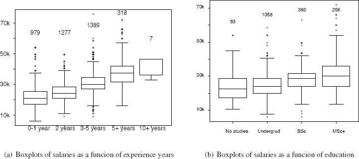
Salary with respect to experience and education, with the number of posts above each box.
As concerns education, Fig. 4(b) shows no particular trend. Although there is some growth with higher education, it is clear that experience is better rewarded, at least in the IT market. Most jobs require at least one year of experience and college/high school or higher education.
3.1. A Regularized Linear Regression Model
Salary is a continuous variable, and it can be estimated through regression. Using regularization methods, it is possible to perform an embedded feature selection and possibly improve the models by avoiding overfitting and selecting the most relevant features.
The raw dataset (as crawled from the web) contains a very large number of features (≈ 2,000), some of which are repetitive or very sparse. Before applying the feature engineering procedure described in the previous Section, one can also keep the original features (properly formatted) to fit a regularized model and observe which and how many variables are automatically removed.
Therefore, we fit a Ridge regression model to the raw features with a twofold objective: providing a simple salary estimation and highlighting the impact of an embedded feature selection.
The optimal value of the regularization constant (C = 4) is found by a 10-fold cross validation. The resulting model contains 487 non-zero coefficients, effectively reducing the number of features. It is evident that the embedded feature selection in this context is not as beneficial in reducing dimensionality as the preprocessing of Section 2, which exploits the domain knowledge. Nevertheless, the resulting R2 obtained for the model is 0.72 on the test set and 0.78 on the overall dataset, thus showing good prediction levels.
3.2. Interpretable Linear Model
Given the set of features in the raw dataset, their contribution to salary prediction is not easily obtained through regularized regression, as each feature’s direct contribution is altered by a set of additional constraints, which are necessary to embed feature selection in the model.
Alternatively, non-regularized linear regression can be employed to provide an estimation of each feature contribution to the model, so as to be able to identify the most relevant features together with the magnitude of their direct contribution. For that purpose, we fit a linear model to the dataset and evaluate the statistical significance of the feature weights by performing two-tailed t tests, in which the null hypothesis corresponds to having a weight equal to zero.
If the corresponding p − values are small enough, one can conclude that there is statistical evidence that the weights are non-zero and that the relative features are relevant for the linear regression. Table 2 displays the top 30 features within the feature set with the highest significance expressed in terms of increasing p-values.
| Estimate | p - value | Estimate | p - value | ||
|---|---|---|---|---|---|
| Intercept | 27,255 | ≈ 0 | Tech. Support | −569 | 2.48×10−06 |
| Experience | 3,295 | 410×10−198 | Angularjs | 494 | 3.23×10−06 |
| Proj. Leader | 1,160 | 1.61×10⁻²⁴ | ASP | −487 | 6.18×10−06 |
| Perm. Contract | 1,157 | 2.68×10⁻²⁴ | Tester | −504 | 8.89×10−06 |
| IT Architect | 1,018 | 3.07×10⁻²² | Windows | −491 | 9.21×10−06 |
| PMP | 911 | 1.61×10⁻¹⁵ | Oracle | −435 | 3.98×10−05 |
| Region | 739 | 3.73×10⁻¹⁴ | JPA | 385 | 6.47×10−05 |
| Hardware | −798 | 3.44×10⁻¹² | BPC | −378 | 6.91×10−05 |
| Operator | −669 | 5.86×10⁻¹⁰ | Helpdesk | −490 | 7.52×10−05 |
| Programmer | −762 | 1.89×10−08 | System | 406 | 0.00022 |
| Office | −523 | 3.14×10−08 | Java | −442 | 0.00023 |
| PHP | −681 | 3.91×10−08 | Sys. Adm. | −461 | 0.00028 |
| Consultant | 598 | 5.65×10−08 | JSP | −357 | 0.00031 |
| Support | −688 | 2.01×10−07 | Open | −346 | 0.00034 |
| Visual Basic | −464 | 3.01×10−07 | Security | 407 | 0.00041 |
Top 30 features according to their significance.
This model is characterized by an intercept whose value is close to the average salary. For each job post, this intercept is modified according to the values of the other features. For instance, a post requiring Consultant and Oracle skills would have a salary equal to the intercept increased by 598 € and reduced by 435 €. Excluding the intercept, there is a significant difference between the top 4 features and the rest of at least seven orders of p-value magnitude, thus suggesting that their values are related or have a bigger influence on the salary. In addition, these features are some of the best paid elements within the job posts, adding more than 1,000 € when present.
The average contribution of features (without intercept) is −24.49, indicating that more requirements imply penalizations rather than gratifications. Indeed, 110 features account for an increase in salary, while 148 for a decrease. Moreover, it is interesting to observe how recent technologies, such as Angularjs or Security, are related to higher salaries, while older and more established technologies, such as Java or Oracle are less demanded and paid.
The coefficient of determination (R2) for this model is 0.57, which is not a good result in terms of predictability of the output. Nonetheless, this simplified model is useful to better understand and interpret the direct impact of each feature and skill on the salary. If interpretability is not the main objective, to increase the prediction accuracy one can fit nonlinear models, as described in Section 4.
3.3. K-means clustering
Clustering algorithms are able to group a collection of samples with numerical attributes according to their distances. Instead of using all possible features within the dataset, here we focus on subsets of relevant variables which divide the job posts in groups according to (i) their job parameters and (ii) skill requirements.
3.3.1. Groups of job posts based on salary and experience requirements
The first grouping scheme relies on features related to salary. We showed previously that there are four features with significant linear dependence on the offered salary, namely Experience, Proj. Leader, Perm. Contract and IT Architect. Apart from showing high p-values in Table 2, these four features are those with the highest correlation with salary. In particular, the correlation coefficient is equal to 0.55 for Experience, 0.31 for Project Leader, 0.26 for Permanent Contract and 0.24 for IT Architect.
We apply k-means clustering to the aforementioned features and the salary variable in order to find groups of job posts containing similar profiles. The use of these features is associated to their potential impact on salary. As a result, there are 9 clusters separating the offers by salary ranges. Table 3 reports the value of the centroids of each cluster sorted by the average salary. Experience is reported as average years, while Project Leader, Permanent Contract and IT architect are expressed as the number of posts in each group.
| # | Size | Salary (€) | Experience (Y) | Project Leader (%) | Permanent Contract (%) | IT architect (%) |
|---|---|---|---|---|---|---|
| 1 | 352 | 13,749.71 | 1.25 | 0.28 | 35.79 | 0.56 |
| 2 | 654 | 19,684.25 | 1.65 | 0.76 | 55.50 | 0.91 |
| 3 | 605 | 23,215.70 | 2.01 | 2.97 | 60.49 | 0.49 |
| 4 | 648 | 26,336.41 | 2.47 | 2.31 | 64.04 | 0.77 |
| 5 | 768 | 29,755.85 | 2.82 | 4.16 | 69.27 | 2.34 |
| 6 | 431 | 34,068.44 | 3.03 | 7.65 | 75.63 | 10.44 |
| 7 | 348 | 39,693.96 | 3.64 | 16.95 | 84.48 | 17.24 |
| 8 | 128 | 48,257.81 | 3.72 | 43.75 | 89.06 | 10.93 |
| 9 | 24 | 63,458.33 | 4.83 | 37.50 | 91.66 | 33.33 |
Cluster centroids.
The resulting groups display linear increments in terms of most features, thus suggesting, as expected, that salary and job conditions mainly improve with experience. Furthermore, the amount of permanent positions increases significantly from early career jobs (low wage, less than two years of experience in average requirement) to established professionals (more than 3 years of experience, higher salaries), suggesting that movement is promoted by companies at early career stages, since experience appears to shape both salary and permanent contract probabilities.
3.3.2. Groups of job posts based on technical skills
Aiming at structuring job posts into a skill-driven scheme, we repeat the k-means clustering experiments using as features only the skill keywords. We obtain 5 clusters of skill-oriented posts, as shown in Fig. 5 along with the top 10 most frequent skills within the posts of each group. This separation scheme shows five well-defined profiles demanded by markets, where different skills provide access to different positions. In this case, the first cluster involves 2,099 posts, the fourth 679, the third 490, the fifth 432 and the second 258. There are different patterns for each of the groups. The first cluster collects several skills typically related to back-end developers and other non-web applications, such as Oracle, SQL, PHP or SAP. The second cluster includes skills required for a Systems Administrator like Linux, Windows, Unix, VMware or Network. The third and fourth clusters include predominantly skills required for .Net developers and Java developers respectively. The fifth cluster corresponds to the most popular technologies for front-end developers.
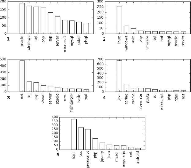
Top 10 skills of each resulting cluster.
From this perspective, it is clear that IT and technology are the most demanded skills by recruiters in Tecnoempleo. Moreover, there are no significant differences in terms of salary as well as experience, with all groups requiring an average experience of two years approximately. This shows the existence of homogeneity across profiles, that is, there appear to be no trending and highly demanded skill sets.
4. Salary range prediction
In order to improve the accuracy of salary prediction, we formulate the problem as a classification task with four classes corresponding to low, medium-low, medium-high and high salary ranges, as described in Section 2. Our experiments compare all the models introduced in the same Section: LM, LR, KNN, MLP, SVM, RF, AB, Vote and Vote3. We use the implementation that is provided by the Python library scikit-learn 49. In particular, we employ several pipelines consisting of 3 main stages:
- 1.
Data normalization to the interval [0,1];
- 2.
Automatic feature selection (optional), which can be helpful in reducing the dimensionality even further than the outcome of our manual feature preprocessing;
- 3.
Classification according to one specific model characterized by the best configuration of parameters as retrieved by applying a previous step of grid search.
To perform the feature selection, we use the X-MIFS algorithm 48 in its original implementation developed by the authors.
4.1. Model configuration and selection
Concerning the (generalized) linear models (GLM), we compare a support vector machine with a linear kernel and LR. The LR models are trained with ℓ1 and ℓ2 regularization with 10 different weights chosen uniformly in the range [10−3,103]. The same regularization scheme is also employed for the SVM, with a maximum number of iterations fixed to 5,000 and a convergence tolerance of 10−3.
For the KNN models, we compare exact algorithms (i.e. with no approximated technique) based on the Manhattan ℓ1-norm distance as well as the Euclidean ℓ2-norm distance. We use two strategies to assign a class to a sample: one that assigns a uniform weight to each neighbour and one that weights the contribution of a neighbour according to the inverse of its distance from the sample so as to give more importance to the closest points. k varied within the set {1,2,4,8,16,32}.
The method used for the optimization of the MLP weights is stochastic gradient descent (SGD). To reduce convergence time an adaptive learning rate is used. In particular, the technique provided by the library is similar to the bold driver method proposed in 50, with the addition of early stopping to avoid overfitting. At each iteration, 10% of the training set is kept apart as a (early stopping) validation set. Starting from an initial value of 1, the learning rate is kept constant as long as the training loss keeps decreasing. Each time two consecutive epochs fail to decrease the training loss or to increase the classification accuracy on the aforementioned validation set by a tolerance value (10−3), the current learning rate is divided by 5. The training stops after a maximum number of epochs (5000) or when the classification accuracy on the validation set does not increase after 50 epochs. The network used for the tests is shallow, with only one hidden layer of neurons and with the tanh activation function. We compare different models with a number of neurons varying in the set {1,2,4,8,16,32} and with 10 ℓ2-regularization weights equally spaced in the interval [10−3,103].
As concerns (non-linear) SVMs, we evaluate models based on radial basis function as well as sigmoid kernels, with a kernel coefficient varying in [10−3,103] and 10 different penalty parameters of the error term taken from the interval [10−3,103]. Even in this case the maximum number of iterations is fixed to 5000 with a tolerance for the stopping criterion equal to 10−3.
Experiments include also RF classifiers trained by using the bootstrap technique. Each tree is trained by using either the Gini impurity criterion or the Information Gain criterion. The number of trees varied in the set {1,2,4,8,16,32}.
The same criteria and number of trees are also employed in the case of the AB classifier. For Vote and Vote3 we use the average predicted probabilities (soft voting) to predict the classes.
For each configuration of the different models, we also investigate the effect of selecting 10 or 20 features (as opposed to considering all the features) by maximizing their mutual information with respect to the class variable.
In order to select the best configuration for each model, we perform a grid search on 90% of the data by using a 3-fold cross validation and by selecting the configuration with the best average classification accuracy. In Table 4 we report the optimal parameters for the different classifiers (excluding the voting classifiers). Note that the use of automatic feature selection is not beneficial. This empirically proves that our customized feature preprocessing already removes (almost) all the possible sources of noise and redundancy through the procedure described in Section 2.
| Pipeline | FS | Model hyper-parameters |
|---|---|---|
| GLM | all | model: LR, regularization: ℓ2, reg. weight: 0.009 |
| KNN | all | distance: ℓ1-norm, k: 8, neighbor weight: distance inverse |
| MLP | all | hidden layer size: 8, reg. weight: 0.001 |
| SVM | all | kernel: RBF, kernel coeff.: 111, reg. weight: 0.009 |
| RF | all | split criterion: Gini, # of trees: 32 |
| AB | all | split criterion: Gini, # of trees: 32 |
Optimal number of features (FS) and model configurations for all the classifiers (excluding Vote and Vote3).
As concerns Vote and Vote3, we do not consider the best configurations of the models individually but we train all the models from scratch and validate the voting classifiers independently from what are the best configurations for GLM, KNN etc. The reason behind this is that the performance of a voting ensemble does not always improve as the performance of the voting members improves. Sometimes weakening one member to decrease its importance in the vote can be beneficial for the final decision. In other cases the difference between two configurations for a single classifier is so negligible that the final vote is not affected at all. This is confirmed by our experiments, with Vote and Vote3 obtaining better accuracy with configurations that are different from those in Table 4. The optimal hyper-parameters for the voting classifiers are reported in Table 5.
| Vote | |
|---|---|
| Model | Hyper-parameters |
| GLM | model: LR, regularization: ℓ2, reg. weight: 0.0045 |
| KNN | distance: ℓ1-norm, k: 16, neighbor weight: distance inverse |
| MLP | hidden layer size: 8, reg. weight: 0.001 |
| SVM | kernel: RBF, kernel coeff.: 111, reg. weight: 0.009 |
| RF | split criterion: Gini, # of trees: 32 |
| AB | split criterion: Gini, # of trees: 32 |
| Vote3 | |
|---|---|
| Model | Hyper-parameters |
| KNN | distance: ℓ1-norm, k: 16, neighbor weight: distance inverse |
| RF | split criterion: InfoGain, # of trees: 32 |
| AB | split criterion: Gini, # of trees: 32 |
Optimal configurations for Vote and Vote3 (differences from Table 4 in bold).
Each model resulting from the grid search is then trained and evaluated on the entire dataset by using 10-fold cross validation.
4.2. Model comparison
The different models and ensembles are compared with respect to the measures described in Section 2. Table 6 summarizes the results for all the classifiers in terms of average accuracy, F1 score, AUC-PR and AUC-ROC, with the indication of the corresponding standard errors. Furthermore, Figures 6–9 provide box plots as well as PR and ROC curves.
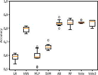
Box plot of classification accuracy.
| Accuracy | F1 score | AUC-PR | AUC-ROC | |
|---|---|---|---|---|
| LR | 0.586 ± 0.0077 | 0.569 ± 0.0085 | 0.603 ± 0.0075 | 0.806 ± 0.0051 |
| kNN | 0.792 ± 0.0067 | 0.792 ± 0.0066 | 0.891 ± 0.0055 | 0.938 ± 0.0034 |
| MLP | 0.591 ± 0.0150 | 0.552 ± 0.0230 | 0.659 ± 0.0110 | 0.831 ± 0.0077 |
| SVM | 0.663 ± 0.0066 | 0.669 ± 0.0076 | 0.881 ± 0.0062 | 0.930 ± 0.0049 |
| AB | 0.836 ± 0.0069 | 0.837 ± 0.0068 | 0.883 ± 0.0060 | 0.936 ± 0.0036 |
| RF | 0.840 ± 0.0076 | 0.838 ± 0.0081 | 0.905 ± 0.0055 | 0.949 ± 0.0028 |
| Vote | 0.844 ± 0.0028 | 0.843 ± 0.0028 | 0.917 ± 0.0036 | 0.960 ± 0.0018 |
| Vote3 | 0.837 ± 0.0073 | 0.837 ± 0.0073 | 0.923 ± 0.0034 | 0.963 ± 0.0017 |
Average scores and standard errors for all the classifiers (best scores in bold).
The classifiers based on ensembles of decision trees (AB and RF) as well as those based on voting ensembles (Vote and Vote3) achieve the best accuracy. Their average accuracy is ≈ 0.84, with the voting classifiers that lead to a slightly better median accuracy (≈ 0.841 for Vote and ≈ 0.85 for Vote3).
It is also evident that Vote is the most robust, since it relies on a larger committee in order to reduce the variance of the final decisions. KNN achieves an average accuracy of ≈ 0.79 and sometimes is comparable to AB or RF. All the remaining models (LR, MLP and SVM) behave significantly worse. For LR, this can be explained by the evident non-linearity of the problem, while for MLP and SVM the scarcity of the data probably represents the biggest obstacle. Note that in the case of the MLP, the best configuration selected 8 neurons and not bigger values such as 16 or 32, thus suggesting that the size of the network is not relevant for the classification.
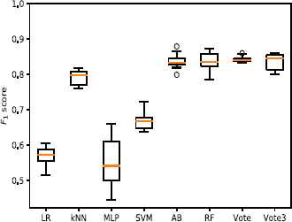
Box plot of F1 score.
The limited set of samples and the categorical nature of most of the features make the MLP and SVM models ineffective. This explains also why the classifiers that can easily deal with categorical features as those based on decision trees (AB and RF) behave generally better. These findings are also confirmed by comparing the models on the F1 score, which accounts for the precision and the recall measures simultaneously. The best average score (≈ 0.843) is achieved by Vote, with RF the second-best (≈ 0.838). The worst results belong to the MLP, which is also the model with the largest variance.
The previous scores describe the performance of each model in recognizing all the classes. In order to get more insight into the capabilities of each classifier, the experiments that led to the results reported in Figures 8 and 9 focus on a slightly different setting.
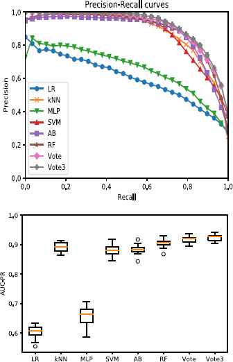
Precision-Recall curves with corresponding AUCs.
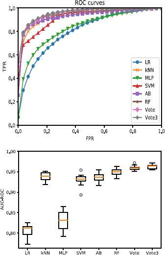
ROC curves with corresponding AUCs.
The same configurations used in the previous tests are employed in a one-vs-rest scenario, in which we compute the precision, recall, true positive rate and false positive rate in the context of a binary classification. For each class, we set to 1 all the members of that class and set to zero all the remaining samples.
We repeat this for all the classes and at the end we average the results obtained. This new setting is interesting because it can describe the behavior of the classifiers with unbalanced classes. It is possible that a model that achieves poor results in the original context is actually better in recognizing one specific class as opposed to all the others.
The best performing models of the previous set of tests continue to achieve the best results also in the new context. However, the SVM performance improves significantly and now is comparable to KNN, AB, RF, Vote and Vote3. This is due to the simplification induced by the new scenario, which is probably characterized by a separating surface that is easier to learn. However, this surface is still non-linear, as it is evident by looking at the poor performance of the LR. The MLP continues to perform poorly even in the new simplified scenario, thus suggesting that the model is not able to extract useful information from the data because of the limited amount of samples. Perhaps deeper architectures are necessary to find more informative features but these models will probably be affected by the scarcity of the data even more.
5. Conclusion
This work focuses on the challenge of predicting the salary offered by companies through job posts on the web. Instead of focusing on international and multi-domain web portals, which are abundant in terms of number of posts, this work analyses job posts collected from Tecnoempleo, an e-Recruitment website specialized in IT jobs for young people in Spain. Domain and geographical restrictions of the website make salary prediction a challenging task. In fact, the number of posts including an explicit indication of the salary, collected in 5 months on a daily basis, is only ≈ 4,000. Moreover, each post is retrieved as a vector of ≈ 2,000 features. From a machine learning perspective, the task is difficult because of the limited number of samples, the relatively high dimensionality and the presence of noise.
After analysing key aspects from the job market, we assess the relevance of the features that can be used to predict salaries. Results indicate that some features, such as experience, job stability or certain job roles (i.e Team Leader and IT Architect) contribute significantly to the final salary perceived by employees.
Furthermore, we observe that posts can be arranged into 5 different skill-based profiles, namely: Back-end developer, Systems Administrator, .Net developer, Java developer and Front-end developer. Such profiles seem to be similarly paid, even though the demand for Back-end developers (including Java and .Net technologies) is higher than that for the rest of professionals.
Finally, this work classifies job posts according to the offered salary range in a noisy and example-scarce context. After collection, features are preprocessed and the dimensionality is reduced by 10 times by using a customized procedure exploiting the domain knowledge. Embedded feature selection or other state-of-the-art filter methods are not beneficial in terms of classification accuracy. We compare several models including logistic regression, nearest neighbors, MLPs, SVMs, random forests, adaptive boosting and voting classifiers based on all or part of them. Experiments show that ensembles based on decision trees behave generally better and that a voting committee based on them leads to an accuracy of ≈ 84%.
Acknowledgments
J. A. Hernández and I. Martín would like to acknowledge the support of the national projects TEXEO (TEC2016-80339-R) and BigDatAAM (FIS2013-47532-C3-3-P), funded by the Ministerio de Economía y Competitividad of SPAIN. The work of A. Mariello and R. Battiti was supported by the University of Trento, Italy.
The work of R. Battiti was also supported by the Russian Science Foundation through the Project entitled Global Optimization, Supercomputing Computations, and Applications under Grant 15-11-30022.
Finally, I. Martín would like to acknowledge the support of the Spanish Ministry of education for financing his FPU grant (FPU15/03518) at Universidad Carlos III de Madrid.
Footnotes
http://www.tecnoempleo.com (last access: June 2018)
See Python’s BeautifulSoup library version 4.4.1, available at http://www.crummy.com/software/BeautifulSoup/ last access: June 2018
The map was generated using Carto: https://carto.com, last access: June 2018
References
Cite this article
TY  - JOUR
AU  - Ignacio Martín
AU  - Andrea Mariello
AU  - Roberto Battiti
AU  - José Alberto Hernández
PY  - 2018
DA  - 2018/07/05
TI  - Salary Prediction in the IT Job Market with Few High-Dimensional Samples: A Spanish Case Study
JO  - International Journal of Computational Intelligence Systems
SP  - 1192
EP  - 1209
VL  - 11
IS  - 1
SN  - 1875-6883
UR  - https://doi.org/10.2991/ijcis.11.1.90
DO  - 10.2991/ijcis.11.1.90
ID  - Martín2018
ER  -