
On-line Evolutionary Sentiment Topic Analysis Modeling
- DOI
- 10.2991/ijcis.11.1.49How to use a DOI?
- Keywords
- topic minding; sentiment analysis; nonparametric Bayesian statistics; Markov chain Monte Carlo
- Abstract
As the rapid booming of reviews, a valid sentiment analysis model will significantly boost the review recommendation system’s capability, and present more constructive information for consumers. Topic probabilistic models have already shown many advantages for detecting potential structure of topics and sentiments in reviews corpus. However, most reviews are presented through time-dependent data streams and some respects of the potential structure are unfixed and time-varying, such as topic number and word probability distribution. In this paper, a novel probabilistic topic modelling framework is proposed, called on-line evolutionary sentiment/topic modeling (OESTM), which has the capacity for achieving the optimization of the aforementioned aspects. Firstly, OESTM depends on an improved non-parametric Bayesian model for estimating the best number of topics that can perfectly explain the current time-slice, and analyzes these latent topics and sentiment polarities simultaneously. Secondly, OESTM implements the birth, death and inheritance for detected topics through the transfer of parameters from previous time slices to the updated time slice. The experiments show that significant improvements have been achieved by the proposed model with respect to other state-of-the-art models.
- Copyright
- © 2018, the Authors. Published by Atlantis Press.
- Open Access
- This is an open access article under the CC BY-NC license (http://creativecommons.org/licences/by-nc/4.0/).
1. Introduction
Reviews imply a lot of valuable sentiment information of consumers on a variety of topics of the product or service. For example, there are praises and complaints over topics, such as the taste of food or the hygiene conditions within restaurant reviews. This information implied within these reviews directly affects the purchase decision-making of consumers. It is more important for company to understand the experience on use of the product, and optimize their produces or services quality. However, it is quite challenging to detect topics and sentiments over the large textual data sets by human being. This has led to the development for the topic-based sentiment mining and retrieval techniques in recent years as a new research field, which aims to automatically detect attitudes and emotions with respect to certain latent topic implied within reviews.
As a core task of topic-based sentiment mining, topic models, that can detect latent topics clustering, have been explored recently. Topic models consist mainly of parametric Bayesian and non-parametric Bayesian methods. Latent Dirichlet Allocation (LDA) 1 is one of the basic and most generally model for parametric Bayesian. LDA extracts and clusters semantically related topics by cooccurrence information of term within a document collection. But LDA can only detect a predefined number of topics. However, reviews often come as time-dependent data streams. The number of topics should be flexibly and automatically learned. So we assume that the number of mixture components (topics) is unknown a priori and is to be inferred from the data. In this setting it is natural to consider sets of Dirichlet process (DP), one for each group, where the well-known clustering property of the Dirichlet process provides a nonparametric prior for the number of mixture components within each group. In this paper, instead of modeling each document as a single data point, we model each document as a Dirichlet process. In this setting, each word is a data point and thus will be associated with a topic sampled from the random measure. The random measure thus represents the document-specific mixing vector over a potentially infinite number of topics. To share the set of topics across documents, Teh et al. introduced the Hierarchical Dirichlet Process (HDP), which is a typical non-parametric Bayesian model and has ability to estimate the best number of mixture components (topics) 2. In HDP, the document-specific random measures are tied together by modeling the base measure itself as a random measure sampled from a DP. The discreteness of the based measure ensures sharing of the topics between all the groups.
But HDP itself is a static model and not considering time-stamp information embed in reviews. If topics are extracted independently through static HDP for each grouped dataset according to time slice, the evolutionary information will be lost. Sentiment analysis also plays an important role in topic-based sentiment mining tasks. Earlier researches mainly use categorization approaches, and have made some achievements. But the basic premise is the need for training data collection, which is based on a substantial amount of time and energy. More importantly, most reviews are not labeled, which puts forward the problem for traditional approaches. The appearance of LDA topic model provides new opportunity for solving these problems. Sentiment analysis approaches based on LDA have the benefit of LDA model, namely that these approaches can train data collection free, and identify topic and sentiment precisely. Meanwhile, these approaches also inherit the disadvantage of LDA model, i.e., the number of topics cannot be learned flexibly and automatically.
Inspired by the above discussions, we propose an on-line evolutionary sentiment/topic model (OESTM) to jointly exploit the sentiment and topics property for continuous reviews. The motivation of OESTM is to detect and track dynamic sentiment and topics simultaneously over time. OESTM has the capacity for estimating the best number of topics through adding a sentiment level to the Hierarchical Dirichlet Process (HDP) topic model, and then control the topics’ birth, death and inheritance by proposed Time-dependent (Chinese restaurant franchise process) CRFP which adds time decay dependencies of historical epochs to the current epochs. Compared with the existing sentiment-topic models, the biggest difference of OESTM is that OESTM can determine topic number automatically. Furthermore, we implement OESTM with the collapsed Gibbs sampling algorithm. The experiment results show that OESTM can effectively detect and track dynamic sentiment and topic.
Compared with the existing methods, the contributions of this work are fourfold:
- •
The proposed OESTM can effectively and jointly exploit the topic and sentiment information of social media reviews.
- •
In order to provide the more flexible method to select the number of topics, OESTM first fuses non-parametric HDP to topic/sentiment analysis model, which models each review document as a Dirichlet Process for topic discovery.
- •
In order to track the evolution of the topics and sentiment, OESTM employs the presented Time-dependent CRFP to accomplish the model’s regeneration.
- •
The main purpose of the sentiment and topic mixture model is to extract the sentiment and topics from social media reviews. We apply our OESTM model to discover the dynamic sentiment and topics with real social media data. We compare the performance of OESTM with ASUM, JST, HDP and LDA. The experimental results show that OESTM outperform these model in terms of generalization performance, model’s complexity, and sentiment classification accuracy, which indicates the effectiveness of our dynamic non-parametric model.
2. Related Work
There are two research fields related specifically to this paper: topic-based sentiment analysis and non-parametric Dirichlet Process. In recent years, a great deal of interest has been attracted to sentiment analysis, as the amount of product/service review grows rapidly. Typical early studies concentrated mostly on sentiment classification, which is composed of detecting opinions and sentiment polarities. Through introducing a method that combined Conditional Random Fields (CRF) and a variation of AutoSlog, Choi et al. implemented opinions and emotions detection 3. Liu et al. presented an analysis framework to compare consumer sentiment polarities score of multiple produces by a supervised pattern discovery method 4.
To determine sentiment polarities of the document, Pang et al. proposed a machine learning method, which adopts text categorization techniques and minimum cuts in graphs 5. In a different study, Pang et al. achieved sentiment classification, where a review can be either positive or negative, at the level of the document using machine-learning techniques via the overall sentiment 6. However, these studies merely focused on to sentiment classification, and did not take the latent topics embedded in the document into account, thus providing insufficient information for consumers, likely leading to inapplicable results. For example, consumers just want to know merits and faults (sentiment) about the battery life (topic) of a cell phone, without having to read an overall product evaluation.
Motivated by this observation, researchers consider combining topic extraction to sentiment analysis, which is called topic-based sentiment analysis. As one of the state-of-the-art methods of topic model, Latent Dirichlet Allocation (LDA) model has gained popularity, which is a hierarchical Bayesian network. LDA builds robust topics’ summaries in accordance with the multinomial probability distribution over words for each topic, and can further deduce the discrete distributions over topics for each document. In order to use time information to improve topics discovery, TOT proposed by Wang et al. models time jointly with word co-occurrence patterns based on LDA in an off-line fashion 7. Meo et al. presented a matching algorithm, that allows dynamically and autonomously managing the evolution 9,8. Nonetheless, above-mentioned topic models have no capabilities of working in an on-line fashion. This stimulated researchers to search for an optimized model, and ultimately several online topic models have been proposed 10,11,12. Using temporal streams information, the dataset is divided by predefined time slice. At each time slice, documents are supposed to be exchangeable. But it is not true between documents across time slice. This core idea will be inherited by this paper. Based LDA and its extended models, many topic-based sentiment analysis models are proposed. Joint sentiment/topic model (JST) 13 and Aspect and sentiment unification model (ASUM) 14 are representatives of these. JST can implement the detection of sentiment and topic simultaneously based on LDA model. ASUM constrains the words in a single sentence to come from same polarity, which is called sentence-level JST model. Since social media data are produced continuously by many uncontrolled users, the dynamic nature of such data requires the sentiment and topic analysis model to be updated dynamically. Time-aware Topic-Sentiment (TTS) 15 and dynamic joint sentiment-topic model 16 are the rarely work to detect and track dynamic topic and sentiment based on probability topic model. However, TTS had jointly modeled time, word co-occurrence and sentiment with no Markov dependencies such that it treated time as an observed continuous variable. This approach, however, works offline, as the whole batch of documents is used once to construct the model. This feature does not suit the online setting where text streams continuously arrive with time.
So far, however, great mass of sentiment analysis models are based on LDA, which also inherit the defect of LDA model that the number of topics must be pre-determined. It is insufficient for the dynamic and massive social media data. The question can be resolved through replacing Dirichlet allocation by nonparametric Bayesian process 17,18,19,20. Dirichlet Process is a typical method for nonparametric Bayesian process, which is represented by DP(G0,α), where G0 is a base measure parameter and α is a concentration parameter. Document could be modeled as a DP, and each word in document d is a target object that is created by the distribution words over a topic sampled from the distribution of document-based mixing vector over infinite number of topics. To allow sharing data among the collection of topics across documents, another non-parametric model, Hierarchical Dirichlet Process, was proposed, which used Dirichlet Processes as the Bayesian prior to solve the topics number determination problem.
Many models that integrating time information based nonparametric Bayesian have recently been proposed to improve topic discovery 21,22. In order to implement dynamically clustering analysis of topics, some nonparametric Bayesian-extended models have been proposed on others 23,24. But, actually there’re several important differences between OESTM and the aforementioned models as following: (1) OESTM is the first dynamic sentiment-topic mixture model based on non-parametric HDP topic model; (2) In order to track the trend of the detected topics, OESTM first uses Time-dependent CRFP to realize the development and change of the topics over time; (3) OESTM implements Gibbs Sampling Process to obtain parameters at each time slice rather than executes global deduction, which is effective for updating timely evolution.
3. Methodology
3.1. Hierarchical Dirichlet Process
Before presenting the on-line evolutionary sentiment/topic modeling (OESTM), let us review the basic Hierarchical Dirichlet Process (HDP). The graphical representations of HDP and OESTM models are shown in Figure 1.
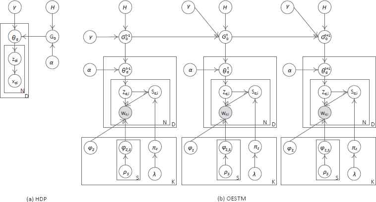
OESTM is shown with one inspiration model: (a) HDP model (b) OESTM model.
HDP (see Fig.1(a)) assumes document as xd with d∈{1,...,D}, and Nd as the size of document d, there is a local random probability measures θd to denote topics distribution of document d. The random probability measure G0 is a global topic distribution shared by all the documents collection, which is distributed as a Dirichlet Process with concentration parameter γ and base probability measure H. Each document d is generated based on local random measures θ that are also distributed as Dirichlet Process and conditionally independent given G0 with concentration parameter α and base probability measure G0. Let kd1, kd2 ... be independent random variables distributed as local measures θ. Each kdi is topic assignment of a single observation ith word within the dth document. Then the word xdi is generated from the conditional distribution F(kdi) given kdi. In order to simplify infer of the sampling process, F is often selected for multinomial distribution, and then forms conjugate distribution with base measure H. The likelihood is given by:
The Hierarchical Dirichlet Process can readily be extended to more than two levels. That is, the base measure H can itself be a draw from a DP, and the hierarchy can be extended for as many levels as are deemed useful. In genefdoral, we obtain a tree in which a DP is associated with each node, in which the children of a given node are conditionally independent given their parent, and in which the draw from the DP at a given node serves as a base measure for its children.
3.2. On-line Evolutionary Sentiment/topic Modeling
While HDP has the capability of determining the appropriate number of latent topics, it is not adequate for tracking the trend of topics; it does not have the capability to combine sentiment labels into training procedure. This stimulates us to propose OESTM (see Fig.1(b)). The reviews dataset x will be divided according to time slice, x = {x1, x2,..., xT}, where T denotes the number of time slices and xt represents the dataset of reviews that included publishing times in the time slice t. Moreover,
In order to further integrate the time information into HDP, base measure G0 should be dynamically calculated for each time slice, that is, the number of mixture components at each time point is unbounded; the components themselves can retain, die out or emerge over time; and the actual parameterization of each component can also evolve over time in a Markovian fashion. Through considering previous time slices, the base measure
The formal definition of the generative process in OESTM model corresponding to the graphical model is as follows:
(1)Generate the global topic distribution at time slice t:
(2)Generate the neural words distribution for each topic: φk ~ H
(3)Generate sentiment words distribution given topic and sentiment:φk,s ~ Dir(ρ)
(4)For each document d:
(4.1)Generate local topic distribution of document:
(4.2)For the ith word in document d:
(4.2.1)Draw an topic assignment:
(4.2.2)Generate sentiment distribution of topic: πz ~ Dir(λ)
(4.2.3)Draw a sentiment assignment: sd,i ~ Mult(πz)
(4.2.4) wd,i ~ φz, φz,s
3.3. Time-dependent CRFP
Chinese restaurant process (CRP) is a metaphor, which is closely connected to Dirichlet Processes, and therefore useful in applications of nonparametric Bayesian methods including Bayesian statistics. CRP is a discrete-time stochastic process, analogous to seating customers at tables in a Chinese restaurant. Chinese restaurant franchise process (CRFP) based on Chinese restaurant process extended Chinese restaurant process to allow multiple restaurants which share a set of dishes, which is a random process that products an interchangeable division of data points and allows multiple data points to share a set of topics 32. CRFP is usually employed to simulate HDP process. In this metaphor each restaurant maintains its set of tables but shares the same set of mixtures. A customer at restaurant can chose to sit at an existing table with a probability proportional to the number of customers sitting on this table, or start a new table with probability and chose its dish from a global distribution. As the expansibility and hierarchy, CRFP is widespread applied in non-parametric models. Although CRFP has the capacity of constructing data point by using a set of topics and allowing topics’ number to be infinite, it is static process and cannot track the development of the latent topics and probability distribution of words. This paper uses CRFP to construct a mixture model of grouped data. However, we replace the first level of CRFP with a novel time-dependent random process. The modified CRFP is called time-dependent CRFP, which can estimate the optimal number of topics for current time slice by considering influences from a previous time slices.
A wide array of metaphors and conceptions are employed in CRFP. An example for time-dependent CRFP is shown in Figure 2. A document is represented as a restaurant, and words are represented as customers in the restaurants. Words that convey homogeneous semantic theme are grouped together as customers of similar taste sit at the same table. A dish is chosen for each table from the global menu of dish tree, which corresponds to topic assignment for each group of words. At restaurant level, each restaurant is denoted by a rectangle and consumers (small circles) sit around different dining-tables (big circles) associated with a dish in this restaurant. At global menu level, the set of dish (topic), is served in common for all of restaurants.
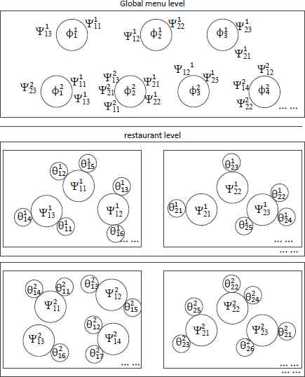
Time-dependent CRFP.
Table assignment
At time slice t, the ith customer comes in restaurant d. This customer can pick jth dining-table with probability:
Dish assignment
We firstly give some notations that will be adopted for dish assignment. Customers in the restaurant sit around different tables and each table is associated with a dish (topic) ψ according to the dish menu (global topics). Let
In order to integrate the historical influences from a previous time slices, another parameter
So the popularity of a topic at epoch t depends both on its usage at this epoch,
If this dish is ordered by consumers in Δ previous time slices but not yet ordered by consumers at t time slice, then changing the distribution of this dish in Markova fashion:
If this dish has not been ordered at any time slices, i.e., it is new dish, then the number of dish Kt increments by one, customer can select a new dish φk ~ H. The probability is as follows:
More formally, getting aforementioned formula together, we have
4. Approximate Posterior Inference
In this section, the collapsed Gibbs sampling algorithm is utilized 25,26 for posterior sampling the assignments of the tables, and the dishes that serve a specific table in each restaurant. For performing Gibbs sampling, Markov Chain Monte Carlo (MCMC) based on time-dependent CRFP is constructed to integrate out parameters
To infer the posterior probability distribution of these, the conditional probability
As base measure H and multinomial distribution (i.e. word distribution with topic) is conjugate distribution, the above formula can be simplified as:
According to time-dependent CRFP and sentiment analysis requirement, we employ the four stages of inference process.
Sampling table b For each customer at time slice t, the distribution of table
Sampling topic k Once the assignment of tables is complete, the posterior sampling dish k can be implemented. The process of sampling dish
Sampling φk Given b, k and observed x, the posterior conditional probability distribution of every φk only depends on whether all consumers enjoyed their dish, which is estimated as follows:
Sampling s Let
OESTM model adopts indirect method of MCMC sampling algorithm to infer distribution parameters θ, φ and π. Using these distribution parameters, the latent topics, the sentiment polarity and represent words of topic can be mined.
5. Experiments
5.1. Datasets Presetting
To accomplish experiments we use two different reviews datasets. The first dataset was composed of restaurant reviews from the website Yelp.com. The second dataset was the collection of hotel reviews that has been used previously 27. These datasets were preprocessed by (1) deleting stop-words and non-English alphabets; (2) deleting low frequency with appearances be low six times, as well as short reviews that are shorter than seven words; (3) adopting Snowball algorithm to stemming for words.
Sentiment analysis is much more challenging than topics detection, because consumers express their attitudes through subtle manner, but topic detection is simply implemented on the basis of words co-occurrence. One technique increasing the accurateness of sentiment analysis is to integrate prior data, i.e., sentiment lexicon. In this section, three sentiment lexicons, Paradiams 28, Mutual Information (MI) 29 and MPQA 30, will be used to improve the sentiment classification accuracy. Table 1 shows the properties of datasets and sentiment lexicon information adopted in our experiments.
| Sentiment lexicon | # of polarity words (pos.neg.) |
|---|---|
| paradiams | 21 / 21 |
| Paradiams/+MI | 41 / 41 |
| MPQA | 1335 / 2214 |
| Corpus | Reviews | Words | Sentences | ||
|---|---|---|---|---|---|
| Restaurant | 41,715 | 3,616,286 | 199,265 Sentence length | ||
| ⩽4 | ⩽12 | ⩽20 | |||
| 26.00% | 79.05% | 93.00% | |||
| Hotel | 34,157 | 4,287,183 | 239,639 Sentence length | ||
| ⩽4 | ⩽12 | ⩽20 | |||
| 34.00% | 82.14% | 95.86% | |||
The properties of the data sets and sentiment lexicon.
Unless otherwise stated, in this experiment these parameters were set according to the following values: the hyper parameter η of base probability measure H was set as 10; concentration parameter γ and α were respectively obtained by vague gamma prior, γ ∝ Γ(1,0.1), α ∝ Γ (1,1). Continuous time slices Δ=4. The number of time slices is set as 20, T=20. To enable comparison to other models, parameters that are LDA-based models were set to the following: Dirichlet hyper parameter α = 0.5,β = 0.02. The hyper parameters λ and ρ were set as 1.0 and {10−7, 0.01, 2.5}. The parameter v in exponential kernel is set as 0.5.
5.2. Perplexity
The density measurement, expressing the potential configuration of data, is the intention of document modeling. Measuring the model’s universal performance on formerly unobserved document is general method to estimate that. Perplexity is a canonical measure of goodness that is used in language modeling to measure the likelihood of a held-out test data to be generated from the potential distributions of the model. In this subsection, we will employ perplexity of the statistical model on test review datasets to measure the generalization performance when the performance of the model starts to steady state. The lower perplexity manifests the better generalization performance will be. We classified the data into 80% for training set and 20% for testing set, where classification proportion is consistently across time slices. Formally, given the testing dataset, the perplexity value can be calculated as follows.
Four models (LDA, ASUM, HDP and OESTM) will be adopted over two datasets to compare the perplexity performance. Firstly, the number of topics for LDA and ASUM was set to 20. The first two rows of Figure 3 illustrate the result of the perplexity as a function of the number of iterations of the Gibbs sampler. Secondly, the number of iterations for four models was set to 100. The second two rows of Figure 3 shows the result of the perplexity as a function of the number of topics. Because nonparametric Bayesian models, HDP and OESTM, are irrelevant to the number of topics, the values of perplexity for them are fixed.
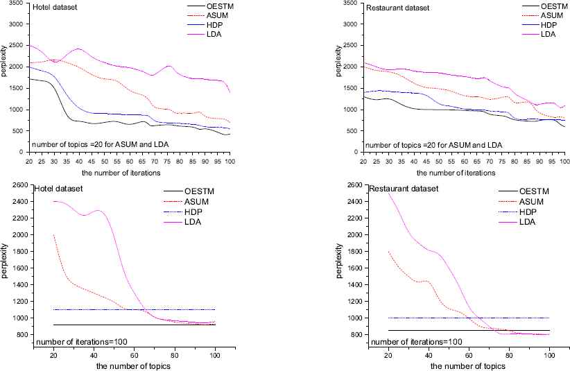
perplexity score on two datasets against different models. The first two rows are perplexity for different numbers of iterations. The last two rows are perplexity for different numbers of topics.
As shown in Figure 3, HDP and OESTM models can effectively work for documents clustering than LDA and ASUM models, i.e., have better generalization performance and presents lower perplexity value. From the results it can also be seen that for LDA and ASUM model, picking the right number of topics is key to getting good performance. When the number of topics is too small, the result suffers from under-fitting. However, blindly increasing the number of topics could on the other hand make over-fitting. On the other hand, the number of topics obtained intelligently under non-parametric OESTM and HDP model is consistent with this range of the best-fitting LDA and ASUM model. Otherwise, OESTM model is slightly better than HDP, which implies that OESTM can well find topics through incorporating information of time and sentiment to provide a better prior for the content of emerging documents. However, perplexity values of OESTM presents overall the similar results with HDP model.
5.3. Complexity
Nonparametric Bayesian methods are often used to sidestep model selection and integrate over all instances (and all complexities) of a model at hand (e.g., the number of clusters). The model, though hidden and random, still lurks in the background. Here we study its posterior distribution with the desideratum that between two equally good predictive distributions, a simpler modelor a posterior peaked at a simpler model is preferred.
In this subsection, we will measure the Complexity of model to evaluate non-parametric Bayesian models 31. To implement the complexity of model the definition of a topic’s complexity will firstly be given. The complexity of a topic is in proportion to the number of words allocated to this topic, i.e., the complexity of a topic is zero if no unique words are allocated to this topic, otherwise, the number of unique words allocated to this topic. So we express the complexity of a topic k as follows:
The complexity analysis considers the number of topics employed to describe the dataset according to Equation 20. A higher complexity of a model shows this model need more topics to express the dataset - that is, the dataset is classified into more dimensions. So a lower complexity manifests the better model will be, on condition that the generated experiment results for perplexity is alike. Figure 4 illustrates the result of the complexity as a function of the number of iterations of the Gibbs sampler for the two different datasets. As shown in Figure 4, OESTM model has lower average complexity and is better than the HDP in all cases. In spite of the advantage of OESTM model in terms of perplexity might be small than HDP, but taking account of average complexity, the overall effect of OESTM model is more superior.
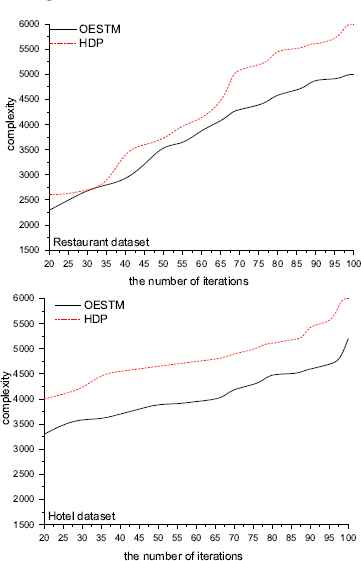
Model complexity comparison of HDP and OESTM models.
5.4. Sentiment Classification
Three sentiment polarity labels, positive, negative and neutral, are selected to associate to all words. l(x) is used to express the polarity label for word x. l(x)=1 if label is positive, −1 negative and 0 neural. Firstly, each word term matches with sentiments lexicon. The sentiment polarity label will be assigned to a word, if that word matches with one of words in sentiments lexicon. Otherwise, a randomly sentiment polarity label from three labels is selected for a word.
After posterior sampling the assignments, i.e., MCMC reaches stead state, each word within a document is attached a sentiment polarity label using a sentiment polarity of a local topic that this word has been assigned. The sentiment polarity of local topics can be further obtained according sentiment distribution π within a local topic. The document sentiment value can be calculated as follows:
Table 2 presents the predictive results of sentiment classification accuracy. It can be observed from Table 2 that through incorporating only 21 pos. and 21 neg. paradigm words, OESTM model merely acquired a relatively poor 74.3% overall accuracy and JST and ASUM acquire 66.8% and 73.5% respectively based on Restaurant dataset. Similar results can be observed for Hotel dataset. By combining the top 20 words based on MI scores with paradigm words, it can be illustrated that there’s lots of improvement in classification accuracy with 2%, 2% and 14% for JST, ASUM and OESTM respectively. But classification accuracy is not proportional to the number of sentiment polarity words. Table 2 shows that incorporating the selected words in the MPQA sentiment lexicon caused the deterioration of classification accuracy, leading to impairment of the performance. Classification accuracy decrease around 1%, 4% and 8% respectively for JST, ASUM and OESTM based on Restaurant dataset. Similar experiment results can be found for Hotel dataset. As shown in it, in all settings, the accuracy of sentiment classification of OESTM model always performs better than JST and ASUM sentiment models.
| Sentiment lexicon |
|---|
| paradiams |
| Paradiams+MI |
| MPQA |
| Dataset | JST(%) | ASUM(%) | OESTM(%) | ||||||
|---|---|---|---|---|---|---|---|---|---|
| Restaurant | pos. | neg. | overall | pos. | neg. | overall | pos. | neg. | overall |
| 63.4 | 70.2 | 66.8 | 70.4 | 76.6 | 73.5 | 70.6 | 78.0 | 74.3 | |
| 70.2 | 78.7 | 74.54 | 74.6 | 84.3 | 79.45 | 86.6 | 88.6 | 87.6 | |
| 68.2 | 78.8 | 73.5 | 72.4 | 80.7 | 76.55 | 78.4 | 84.7 | 81.55 | |
| Dataset | JST(%) | ASUM(%) | OESTM(%) | ||||||
|---|---|---|---|---|---|---|---|---|---|
| Hotel | pos. | neg. | overall | pos. | neg. | overall | pos. | neg. | overall |
| 66.6 | 74.6 | 70.6 | 68.3 | 75.4 | 71.85 | 71.4 | 78.8 | 75.1 | |
| 72.3 | 80.7 | 76.5 | 76.4 | 86.5 | 81.45 | 87.9 | 89.6 | 88.75 | |
| 68.6 | 79.8 | 74.2 | 72.4 | 81.4 | 76.9 | 74.6 | 86.7 | 80.65 | |
Sentiment classification accuracy comparison.
5.5. Hyperparameter Sensitivity
There are two principle parameters defined in OESTM model, namely ν and η, where ν defines the time decaying kernel, and η is the hyper parameter of base probability measure H. To assess the sensitivity of OESTM to hyper parameters’ settings, we conducted a sensitivity analysis in which we hold all hyper parameters fixed at their default values, and vary one of them. Held-out likelihood (LL) is widely used in the topic modeling community to compare how well the trained model explains the held out data. In this subsection, we use parameter variations as a proposal for calculating the test LL based on Restaurant dataset for OESTM. We should note here that the order of the process can be safely set to T, however, to reduce computation, we can set Δ to cover the support of the time-decaying kernel, i.e, we can choose Δ such that E(ν, Δ) is smaller than a threshold, say .001. The results are shown in Figure 5.
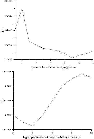
Held-out Likelihood for different parameters.
Firstly, While varying ν, we fixed Δ = T to avoid biasing the result. We noticed that when ν = 6, some topics weren’t born and where modeled as a continuation of other related topics. ν depends on the application and the nature of the data. In the future, we plan to place a discrete prior over ν and sample it as well. Secondly, the best setting for the variance of base measure is from [5, 10], which results in topics with reasonably sparse word distributions.
5.6. Evolutionary Senti-Topic Discovery
OESTM is proposed to produce topics coupled with a sentiment for each time slice, easier facilitating customers to reveal how development and change of topics and topic sentiment scores developed over time. In this experiment, the probability distribution for words given topic k, i.e. neural words that are assigned to topic k was estimated using φk, the distribution for words given topic k and sentiment label s was estimated using φk,s. In order to track the sentiment trend for each topic, the sentiment scores of topic k with sentiment polarities for time slice t are defined as following.
In this subsection, the topic word probability distributions and the sentiment word probability distributions of topics for different time slice will be firstly obtained by OESTM. Then each topic’ sentiment score for different time slices will be calculated through equation 23. Four example topics were used: the first three are selected by the probability values, ranging from high to low, while the last one is selected randomly. This is coupled with topic and senti-topic words probability distributions of three time slices in the left of Figures 6 and 7. The first five topic words and ten senti-topic words are picked attached probability. The emotional changes of left four topics, reflected by sentiment score, for different time slices are shown at the right of Figure 6 and Figure 7.
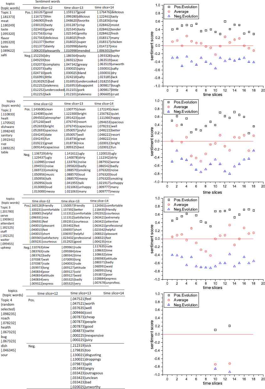
Evolutionary senti-topic discovery based on Restaurant dataset.Left are discovered topics, topic words and senti-topic words. Right are the sentiment emotional changes of left topic.
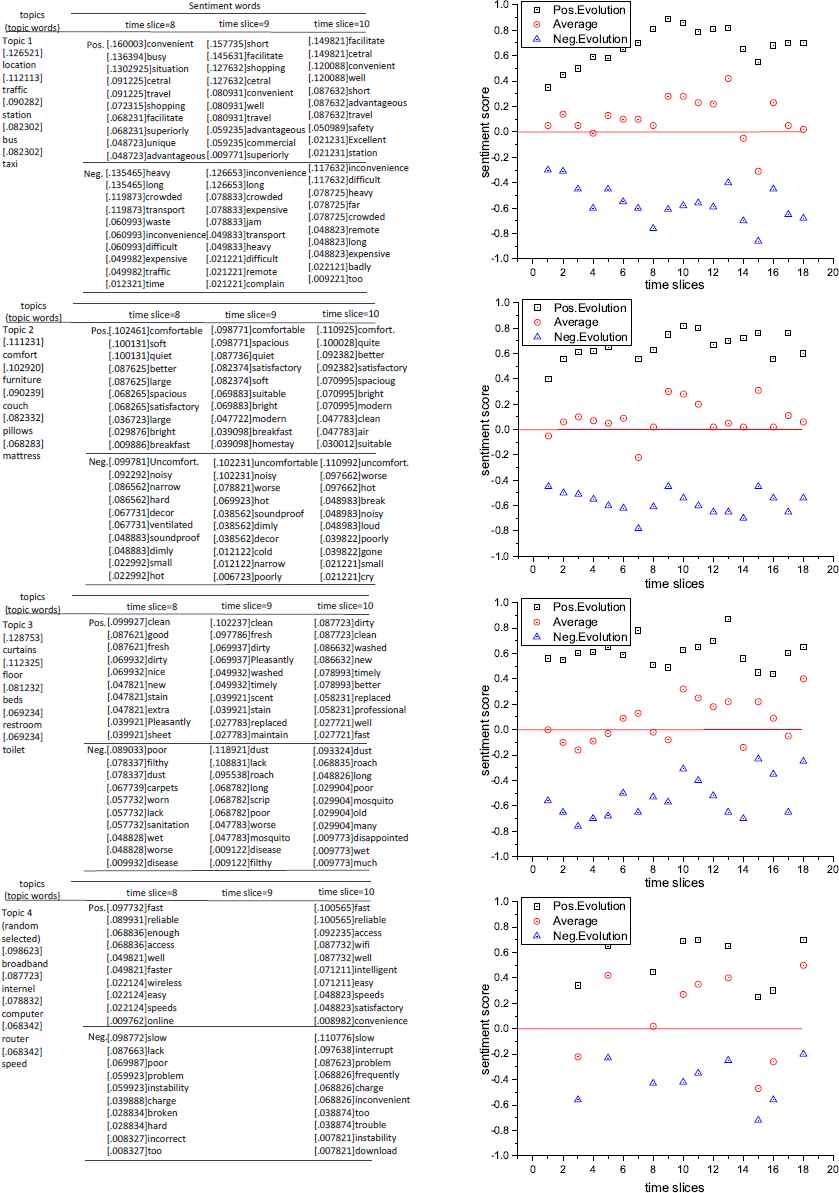
Evolutionary senti-topic discovery based on Hotel dataset.Left are discovered topics, topic words and senti-topic words. Right are the sentiment emotional changes of left topic.
For example, the first topic word for the extracted topic 1 based on Restaurant dataset is “meat” with probability 0.181373, and the senti-topic words coupled with positive and negative label at time slice 12 are “good” and “dry” with probability 0.161267 and 0.152256 respectively. Topic 4 based on Restaurant dataset is emerging at time slice 10, which is inherited at time slice 13. After time slice 13 this topic is not be identified and will die at time slice 13+Δ. This proves the efficacy of OESTM in achieving the birth, death and inherit of topics. The topic 4 based on Hotel dataset is born at time slice 3, which is observed from sentiment score graph, but do not been identified at time slices 4, 6, 9, 14 and 17. This topic has no died, because it is used for subsequent consecutive Δ time slices, rather than been inherited through considering influence from previous time slices to the updated time slice at time slices 5, 7, 8, 10, 11, 12 and 13. This proves more that our proposed model has capacity to inherit topics that are identified at previous consecutive Δ time slices.
The sentiment score reflects the topic’ emotional status. For example, the sentiment average score for topic 2 based on Restaurant dataset at time slice 7 is −0.49, which indicates that a lot of negative feedback during this period on health topic have been received. This can attract the attention of the company, and supervise and urge it to improve related service.
6. Conclusions
In this paper we addressed the problem of modeling time-dependent review corpus. On-line evolutionary sentiment/topic modeling (OESTM) is proposed, which can adapt number of topics, the topic words (without sentiment information) distributions of topics, the senti-topic words (attached sentiment polarity labels) distributions of topics, and track the topics’ emotional development over time slice. As far as we know, we are the first to deal with a time-dependent reviews through non-parametric Bayesian topic model in order to implement topic-based sentiment analysis. At each time slice, a topic-clustering with the estimated best cluster number based on time-dependent CRFP, smoothing with the topics’ inheritance by considering historical influences from a previous time slices and sentiment analyzing for latent topics are automatically implemented. A collapsed Gibbs sampling algorithm is utilized to infer parameters. To evaluate the effectiveness of our proposed algorithm, we collect a real-world dataset to conduct various experiments. The preliminary results showed superiority of our proposed model over several state-of-the-art methods on generalization performance, lower complexity, accurate sentiment classification.
One of the limitations of our model is that it requires setting the time span of each epoch. In the future, we will consider other time dependency modes to optimize dynamic parameter inference.
Acknowledgments
This work is supported by the National Natural Science Foundation of China No.61303131, No. 61672272, No. 60973040;
Cite this article
TY  - JOUR
AU  - YongHeng Chen
AU  - ChunYan Yin
AU  - YaoJin Lin
AU  - Wanli Zuo
PY  - 2018
DA  - 2018/01/22
TI  - On-line Evolutionary Sentiment Topic Analysis Modeling
JO  - International Journal of Computational Intelligence Systems
SP  - 634
EP  - 651
VL  - 11
IS  - 1
SN  - 1875-6883
UR  - https://doi.org/10.2991/ijcis.11.1.49
DO  - 10.2991/ijcis.11.1.49
ID  - Chen2018
ER  -