
Why Linguistic Fuzzy Rule Based Classification Systems perform well in Big Data Applications?
- DOI
- 10.2991/ijcis.10.1.80How to use a DOI?
- Keywords
- Big Data; Fuzzy Rule Based Classification Systems; Interpretability; MapReduce; Hadoop
- Abstract
The significance of addressing Big Data applications is beyond all doubt. The current ability of extracting interesting knowledge from large volumes of information provides great advantages to both corporations and academia. Therefore, researchers and practitioners must deal with the problem of scalability so that Machine Learning and Data Mining algorithms can address Big Data properly. With this end, the MapReduce programming framework is by far the most widely used mechanism to implement fault-tolerant distributed applications. This novel framework implies the design of a divide-and-conquer mechanism in which local models are learned separately in one stage (Map tasks) whereas a second stage (Reduce) is devoted to aggregate all sub-models into a single solution. In this paper, we focus on the analysis of the behavior of Linguistic Fuzzy Rule Based Classification Systems when embedded into a MapReduce working procedure. By retrieving different information regarding the rules learned throughout the MapReduce process, we will be able to identify some of the capabilities of this particular paradigm that allowed them to provide a good performance when addressing Big Data problems. In summary, we will show that linguistic fuzzy classifiers are a robust approach in case of scalability requirements.
- Copyright
- © 2017, the Authors. Published by Atlantis Press.
- Open Access
- This is an open access article under the CC BY-NC license (http://creativecommons.org/licences/by-nc/4.0/).
1. Introduction
Big Data is nowadays more than just a buzzword. It stands for the opportunity of addressing large volumes of information to gather the highest value from it1. However, standard learning methodologies for data modeling are no longer capable of addressing this task. The cause of this problem is the lack of scalability2. This fact is translated into longer training times, or may even make impossible to cope with such data with traditional implementations.
The aforementioned issue implied the migration towards a novel framework from which Data Mining algorithms are able to use the whole dataset in a reasonable elapsed time3. This framework is known as MapReduce4, and it mainly consists of two processes: (1) Map, that divides the computation into several parts, one devoted for a different chunk of the total data; and (2) Reduce, that aggregates the partial results from the previous stage. By implementing these two processes, any algorithm will be automatically distributed in a transparent way, and it will be run within a fault-tolerant scheme.
In this work, we focus on the classification task for Big Data problems, and more particularly on linguistic Fuzzy Rule Based Classification Systems (FRBCS)5. This type of models are considered an effective approach to model complex problems. In particular, when tested in the context of Big Data, they have excelled as an accurate and recommendable option6,7.
Due to this good behavior, in recent years the interest of researchers in this topic has significantly increased. We may find several works in different contexts such as classification 8, regression 9, and subgroup discovery 10.
However, the reasons behind this good behavior have not been investigated yet. Therefore, in this contribution we aimed to answer one “simple” question: why do FRBCSs perform well in Big Data problems? To reach this objective, we will provide several hypothesis regarding different capabilities related to the learning scheme of linguistic FRBCS:
- (a)
FRBCS are a robust approach when facing the lack of data problem with respect to other paradigms of classification. Specifically, we state that they can be able to model accurately a given dataset even in the case of mining only a subset of the original11. This fact is of extreme importance when scalability is seek in MapReduce models, i.e. when increasing the number of maps to address the learning task. Finally, we consider that the aggregation of the local models learned within each Map is important for reaching a high performance.
- (b)
As the number of maps increases, the size of the local rule bases becomes smaller. This implies three issues. (a) First, we may state that these models may comprise a higher interpretability. (b) Second, more diversity between these rules bases is expected, measured in terms of different antecedents. (c) Finally same antecedents may be found along different maps but associated with different consequents. These facts enrich the aggregation step during the Reduce task, leading to a precise fuzzy model.
- (c)
Rules contribute in a different degree during the classification stage. Considering an inference mechanism based on the “winning rule,” i.e. the one rule with the highest activation degree determines the output label, just a subset from the total fuzzy rules will be used in the decision stage. This issue is mainly caused by the fuzzy overlap among rules, i.e. different rules cover the same problem space. In addition, rules with a higher support are expected to be selected more often than those associated with few training instances. However, this latter type of rules are also of importance, as they cover those instances far from the high density areas of the problem.
To contrast whether these hypothesis are actually fulfilled, we will carry out an experimental study making use of Chi-FRBCS-BigData12, being the first linguistic FRBCS that was adapted to the MapReduce scheme. In summary, we will analyze the differences in performance with respect to the lack of data for the learning stage, how rules are distributed among Maps, and their impact into the classification stage.
To carry out this research, this document is divided as follows. In Section 2 we describe the main components and procedure of Chi-FRBCS-BigData, and then we discuss some of the properties that may be associated with the good behavior of FRBCS in Big Data problems. Section 3 contains the experimental framework to carry out our experiments. Section 4 is devoted to investigate the behavior of FRBCS within a MapReduce execution environment. Section 5 analyzes some additional capabilities of fuzzy models for Big Data applications, such as the rule repetition, double consequent rules, and the influence of the fired rules. Once the hypotheses established in this paper have been contrasted, we develop a summary of the lessons learned and we provide some topics for future work in Section 6. Finally, Section 7 presents the conclusions and future work on the topic.
2. Fuzzy Rule Based Classification Systems for Big Data
In this research work, we aim to answer several questions related to the good behavior observed for FRBCS in Big Data problems. To do so, we first introduce in Subsection 2.1 the Chi-FRBCS-BigData algorithm that will be used as a baseline approach for our experiments. Then, we enumerate some of the positive aspects of linguistic fuzzy systems for classification tasks in Subsection 2.2.
2.1. Chi-FRBCS-BigData: a grid-based algorithm for Big Data
In this work, we will make use of linguistic FRBCSs5. They are composed of a Knowledge Base (KB), including both the information of fuzzy sets (stored in a Data Base (DB)) and rules (within a Rule Base (RB)), and an inference system. Specifically, the DB will be obtained ad hoc by means of linguistic fuzzy labels (triangular membership functions) homogeneously along the range of each variable. The RB will be extracted using a learning procedure from training examples.
To address Big Data problems, we have selected the pioneer fuzzy rule learning algorithms in this context, Chi-FRBCS-BigData12. As its name suggests, this method was based on the Chi et al.’s approach13, adapting their implementation into a MapReduce work-flow. The advantages of using such a linguistic model is having the same rule structure and DB for all the distributed subprocesses, thus simplifying the whole design.
In Chi-FRBCS-BigData the initial dataset is divided into several chunks of information which are then fed to the different Map functions. Afterwards, the obtained results are simply aggregated within the Reduce functions. The whole procedure, which is summarized in Figure 1, consists of the following stages:
A workflow of how the building of the KB is organized in Chi-FRBCS-BigData.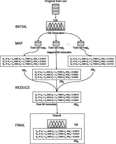
- (a)
Initial: the DB is built computing homogeneous fuzzy partitions along the domain of each attribute, depending on the level of granularity selected. Next, the whole training set is divided into independent data blocks which are transferred to the processing units together with the common fuzzy DB.
- (b)
Map: In this stage, each processing unit works independently over its available data to build its associated fuzzy RB (noted as RBi in Figure 1) following the original Chi-FRBCS method13.
Specifically, the procedure iterates among all examples, deriving all possible sets of antecedents taking those fuzzy labels that give the highest membership degree per example. To assign a single consequent for each antecedent that was previously obtained, Rule Weights (RWs) are computed by means of the Penalized Certainty Factor (PCF) 14 shown in Equation (1). RWs measure the fuzzy degree of confidence of a rule for its area of influence, i.e. the “fuzzy” proportion of covered examples with the same label of the consequent part of rule. To do so, for a rule j, the membership degree values μAj(xp) are computed for each covered training example xp (denominator part). These values are obtained by considering the matching degree of each attribute of xp with the antecedent of the rule, and combining these values via a t-norm. In the numerator part, the previous sum is divided into two parts, one considering those examples with the same class label of the consequent of the rule Cj, and the other part for the remaining examples. This way, RWs will be tend to zero (or even negative) in case of covering many examples from other classes at a high degree. Final class label is set as the one resulting on the greatest RW.
- (c)
Reduce: In this third phase, all RBi computed by a Map process are aggregated to obtain the final RB (called RBR in Figure 1). As rules with the same antecedent may come from different Maps, we follow the Chi-FRBCS-BigData-Avg scheme in which the final RW is computed as the average of those of the rules of the same consequent. In case of having rules with identical antecedent and different consequent, the one with the highest RW is maintained in RBR.
- (d)
Final: results computed in the previous phases are provided as the output of the computation process. The generated fuzzy KB is composed by the fuzzy DB built in the “Initial” phase and the fuzzy RB, RBR, obtained in the “Reduce” phase. This KB will be the model that will be used to predict the class for new examples.
2.2. Discussing the capabilities of linguistic FRBCSs
In this section, we want to stress some of the properties that allow linguistic FRBCS to be an accurate solution in a general context of classification. By understanding the basis of the use of linguistic labels and membership functions, as well as the nature of the inference process, we can be able to analyze the way these features affect positively when addressing Big Data problems. We provide a description of these issues throughout the following items:
- •
The universe of discourse of fuzzy membership functions is defined all along the range of the input attributes. Furthermore, the lower the granularity selected for the fuzzy partitions, the higher the area of coverage of a single label. In this sense, during the learning step just few examples are needed to discover a new rule. The only requirement is that the example attribute values were set under the influence area of a new fuzzy label, i.e. the membership degree is above 0.5. This is how linguistic FRBCS cope well with the lack of data, whenever the training examples are uniformly distributed along the problem space.
- •
The advantages of linguistic fuzzy labels are not only related to the learning step. During the classification task it is probable that just few linguistic fuzzy rules are needed to represent accurately the whole problem space. This is due to the high support associated with each fuzzy rule, especially in the case of datasets with a low number of attributes, or when “don’t care” labels are allowed within the antecedent.
- •
Support and confidence of fuzzy rules are two features with a significant influence for the success of an FRBCS. As stated previously, the higher the support of the rules that compose the RB, the compacter the RB becomes. This fact is positive for the interpretability of the system, but also probably for its generality and therefore its accuracy. Regarding the confidence of the rules, mainly computed and integrated as the RW14, we must state that it is a component that allows for the smoothness of the borderline areas of each rule, especially in the event of overlapping. Therefore, the joint of support and confidence of a fuzzy rule stands for their classification skill.
- •
Finally we must analyze the influence of the fuzzy inference process on the robustness of FRBCS, which summarizes all the advantages of the previous analyzed components. First, we must acknowledge that during the whole inference many rules can be fired at different degrees, depending on their coverage of the example measured in terms of membership degrees, and aggregated via t-norms. Therefore, for a single input example there will be many candidate rules, possibly with contradictory consequent values. The key here is, as stated above, the combination between the aggregated membership degree and the rule weight. High confidence rules, that were learned in a non-overlapped area, will have prevalence, as they will be given a higher value. Finally, if we consider a “winning rule” fuzzy reasoning method, two advantages arise: on the one hand, we delimit an specific activation area by considering only the most significant rules per class; on the other hand, we are able to explain the phenomena related to the problem by simply interpreting the antecedents of the finally selected fuzzy rule.
3. Experimental Framework
In this section, we introduce our experimental framework in which the details of the benchmark datasets and the parameters are given.
For this study, we have selected three Big Data problems from UCI repository15: Covtype, Poker and Susy datasets. These problems are translated into binary datasets by joining pairs of classes or contrasting one class versus the rest. A summary of the problem features is shown in Table 1, where the number of examples (#Ex.), number of attributes (#Atts.), selected classes, and number of examples per class, are included. Table is in descending order according to the number of examples of each dataset.
| Datasets | #Ex. | #Atts. | #Samples per class |
|---|---|---|---|
| Covtype_1_vs_2 | 495,173 | 54 | (211,705; 283,468) |
| Poker_0 | 1,025,009 | 10 | (513,701; 511,308) |
| Susy | 4,923,622 | 18 | (2,711,811;2,211,811) |
Summary of BigData classification problems.
For the experimental analysis, we will take into account the accuracy metric to evaluate the classification performance. The estimates for this metric will be obtained by means a 5-fold stratified cross-validation partitioning scheme.
The configuration parameters for Chi-FRBCS-BigData algorithm are presented in Table 2 being “Conjunction operator” the operator used to compute the compatibility degree of the example with the antecedent of the rule and the operator used to compute the compatibility degree and the RW. We must recall that regarding the “Reduce” stage we will make use of the Chi-FRBCS-BigData-Avg version, as stated in Section 2.
| Number of Labels: | 3 fuzzy partitions |
| Conjunction operator: | Product T-norm |
| Rule Weight: | Penalized CF14 |
| Fuzzy Reasoning Method: | Winning Rule |
Configuration parameters for Chi-FRBCS-BigData.
Regarding the infrastructure used to perform the experiments, we have used the research group’s cluster with 16 nodes connected with a 40Gb/s Infiniband. Each node is equipped with two Intel E5-2620 microprocessors (at 2 GHz, 15MB cache) and 64GB of main memory running under Linux CentOS 6.6. The head node of the cluster is equipped with two Intel E5-2620 microprocessors (at 2 GHz, 15MB cache) and 96GB of main memory. Furthermore, the cluster works with Hadoop 2.6.0 (Cloud-era CDH5.4.2).
Finally, with aims at analyzing the differences of the performance and KB components under different levels of scalablity, we have selected a wide number of Maps for the data distribution. Specifically, we have run Chi-FRBCS-BigData with 1 (sequential version), 8, 16, 32, 64 and 128 Maps.
4. An Analysis on the Reasons for the Good Performance of Linguistic Fuzzy Rule Based Classification Systems in a MapReduce Execution Environment
This section is devoted to study the components and capabilities of FRBCS in a Big Data scenario. To do so, we divided it into two parts. On the one hand, to determine the robustness in terms of relative performance for FRBCSs when increasing the number of Maps. This implies the seek for a higher level of scalability in the computation (Subsection 4.1). On the other hand, to analyze the components of the RB in the MapReduce workflow, focusing on the distribution of rules along the Map tasks (Subsection 4.2).
Our ultimate goal is to analyze whether there is a trend with respect to the degree of scalability, i.e. number of Maps, and to provide a better insight on the how we might obtain the highest benefit from Big Data using fuzzy systems.
4.1. Are FRBCSs robust with respect to the lack of data?
For this first task, we will analyze the behavior of FRBCSs with respect to the lack of data. Our objective is to establish the goodness of the local models learned within the Maps, disregard the number of distributed tasks. To do so, we carry out a comparison of the accuracy obtained by Chi-FRBCS-BigData and a sequential run of Chi (named as Chi Standard).
We must recall that in the first case (Chi-FRBCS-BigData), the whole MapReduce procedure is executed, i.e. a local RB is learned within each Map procedure and results are then aggregated in the Reduce step. On the contrary, for Chi Standard we emulate the behavior of running a single Map, i.e. we learn the fuzzy model using just a subset of the initial training data.
This analysis is illustrated in Figure 2, where we depict the accuracy values achieved in the three selected problems. Graph bars are grouped by pairs, so that each couple corresponds to the comparison between Chi-FRBCS-BigData (noted as ChiBD for short) and Chi Standard (ChiStd) in one particular problem. Results are divided by the number of maps, from 1 Map (100% of the problem is used for training) and 128 Maps (1% approximately of the original problem).
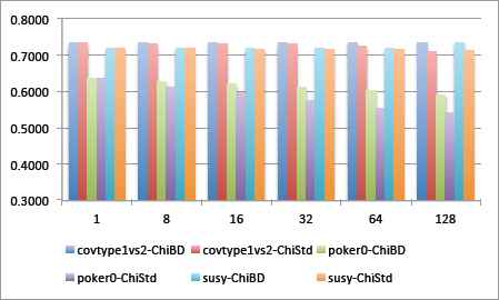
Accuracy comparison between Chi-FRBCS-BigData (ChiBD) and Chi Standard (ChiStd) with respect to different number of Maps in covtype1_vs_2, poker0 and susy datasets.
We may observe that the performance is stable in both cases (Chi Standard and Chi-FRBCS-BigData) even when using more Maps. We must point out that there is a dependency of the problem, as the ratio of loss is a bit higher for the “Poker0” dataset.
In order to carry out a more detailed analysis, we show three additional accuracy graphs in Figure 3, one per benchmark problem. In this comparison, we have also included the results of the C4.5 decision tree16. Our objective is to contrast whether FRBCS are actually more robust to the lack of data than other state-of-the-art rule-based learning classifiers. Bar graphs are computed taking into account the relative differences (in percentage) of each classifier in test with respect to the baseline case, i.e. when the whole dataset is used. We must make clear that for this study the data has been divided at random, i.e. no informed prototype selection of the data has been carried out to achieve a better representation of the initial problem.
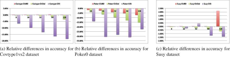
Variation of accuracy (in percentage) with respect 1 Map (100% training set) from 8 to 128 Maps. Algorithms represented: Chi-FRBCS-BigData, Chi standard algorithm and C4.5.
We may observe that the performance is stable in both FRBCSs (Chi Standard and Chi-FRBCS-BigData) as data is decreased from each case study (when using more Maps). We must point out that there is a dependency of the problem, showing a very small ratio of loss for Covtype1_vs_2 and Susy, but being a bit higher for the “Poker0” dataset, i.e. up to 7% for Chi-FRBCS-BigData, and 15% for Chi Standard.
Two clear conclusions can be extracted from this analysis. On the one hand, the advantage of aggregating the local models in the MapReduce methodology must be emphasized (for Chi-FRBCS-BigData), as a lower percentage is loss in all cases, or even better results are achieved (Susy with 128 Maps). On the other hand, the differences in percentage between Chi Standard and C4.5 are very clear for all problems, especially for Covtype1vs2.
Taking into account these findings, we may conclude that FRBCSs based on linguistic labels are able to provide accurate models even in the scenario of lack of data.
The reason is clear, as it was exposed in Section 2.2. As fuzzy labels cover the whole range of the input data attribute values, only few examples are needed to derive fuzzy rules that actually represent a higher region, i.e. those whose membership function computation is above 0.5. The only issue in this case is being able to provide a precise computation of the rule weights, i.e. the confidence related to each rule.
4.2. Analysis of the RBs along Map tasks
In this part of the study, we will consider the relationship between the number of maps and the composition of the individual RBs that are generated during the learning process. We aim to identify whether there are significant differences regarding three issues, namely the number of rules in the final RB, the contribution of each map to the final RB, and how many rules are removed due to a negative RW.
- •
Final number of rules: In Figure 4 we show the total number of rules from 1 Map (sequential approach) to 128 Maps (MapReduce approach).
We can observe that, as we increase the number of Maps, so does the number of final rules that compose the RB. Actually, the same rule antecedents are always generated disregard the number of Maps, as the Chi method obtains one rule per example.
The issue observed in this case can be explained if we focus on the P-CF RW computation. In this case, rules with a negative value are removed from the local RBs. When the amount of data diminishes in the learning stage, it is less probable that the number of negative-class examples for a given rule, i.e. those with contrary class label, appear in the activation area of the rule.
We observe an exception in the case of the Susy problem with 128 Maps, which is due to significant decrease in the number of rules for the first class. Specifically, in this case 1700 rules have been mined for the first class, versus 6072 for the second one. In the remaining cases (1 to 64 Maps) these values are about 2100 and 6000 respectively. The most straightforward explanation is that examples of the first class are located within small disjuncts and overlapping areas17. This inner characteristic of the data causes the contrary effect of what was described previously. This fact will be analyzed in the next item of study.
- •
Rules removed in Map: To carry out this analysis, Figure 5 shows the percentage of rules that are discarded prior to the reduce stage per Map, with respect to the total number of rules discovered in the learning process.
As we may observe from these graphs, when the data is sparsely distributed (more maps are selected) the values of the RWs become higher. This is an expected behavior as the less examples considered, the lower possibility of overlap among them. As a result, more rules are generated (as shown in the previous item), although the RW computation probably differs from the actual one.
When studying the final number of rules, we pointed out that the relationship between the number of Maps and rules in the final RB was directly proportional. The exception for the Susy dataset is now properly explained, as it follows the contrary trend than the two other case studies. As commented before, several instances may be located within small disjuncts that are highly accentuated when increasing the data distribution.
- •
Rules generated per Map: In this last item, we will study how each Map (RBi) contributes to the RB. With this aim, Figure 6 shows, for each value of the “map” parameter, the percentage of rules from a single map that are finally stored. Therefore, it is the average of rules among maps, divided by the total amount of rules.
The results are quite similar for the three problems studied. The trend is clear: the higher the number of maps, the smaller the contribution of each RBi. Obviously, as fewer data is fed for the learning stage, the RBs become also smaller. This fact implies a better interpretability within each local fuzzy classifier, whereas its accuracy is somehow maintained as shown in Subsection 4.1. Indeed, few fuzzy rules are necessary to provide a good representation of the global problem space.
A complementary analysis is shown in Figure 7, where instead of the percentage of contribution of each RBi to the final RB, we illustrate the average number of rules generated within each Map task. The trend is similar to the one shown in Figure 6, that is, the higher the selected Maps, the lower the number of rules per Map. Finally, when all RBi are aggregated in the Reduce step, the global RB is composed by a larger number of fuzzy rules (see Figure 4).
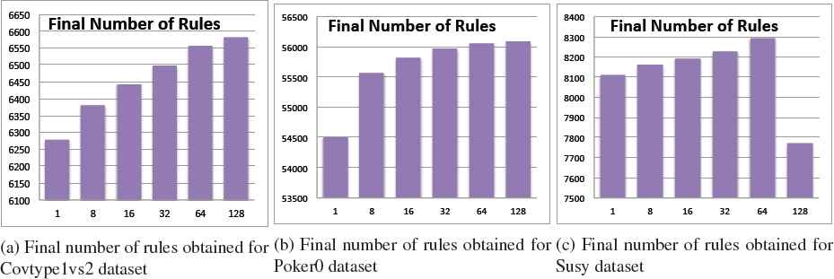
Final number of rules obtained for Chi-FRBCS-BigData under different number of Maps.
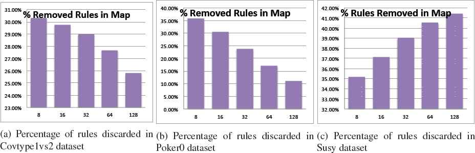
Percentage of rules discarded due to a negative RW in the Map task.
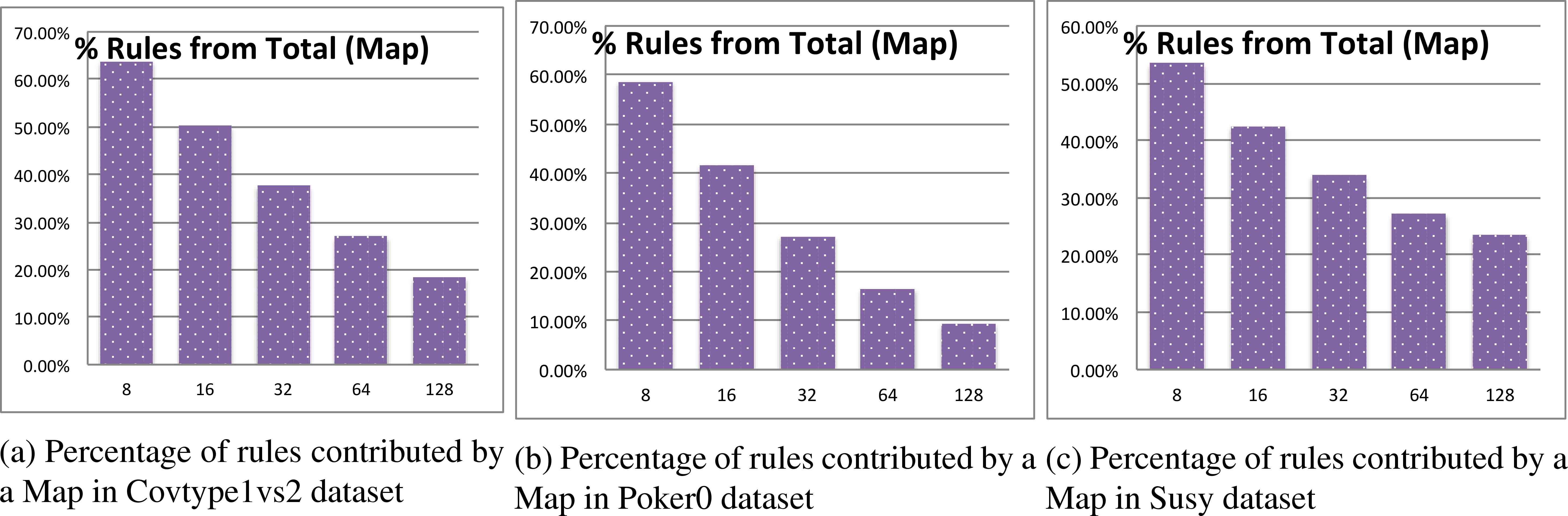
Percentage of rules from each map (RBi) that are stored in the final RB.
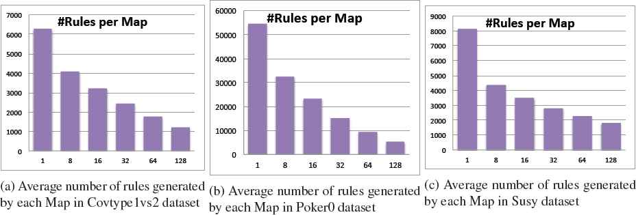
Average number of rules obtained by each map (RBi).
5. Analysis of Additional Capabilities for Fuzzy Models in Big Data
In this section, we will study more specific issues about the components of fuzzy models in Big Data. Specifically, we will first focus on the rules that are fed to the Reduce tasks, considering different characteristics such as the rule repetition (same antecedent), and double consequent rules (Section 5.1). Then, we will analyze the contribution of the discovered fuzzy rules in the final classification stage (Subsection 5.2).
5.1. Distribution of fuzzy rules along Reduce tasks
During the MapReduce workflow of the Chi-FRBCS-BigData algorithm, rules discovered in each map are collected using their antecedents as “key” for the reduce stage. Therefore, reducers are responsible for carrying out the fusion of all rules by aggregating those that came along with the same key, i.e. antecedent.
We may observe three particular cases of use. First, we can determine the amount of rules with identical antecedent generated by different maps. Second, from the previous rules, some of them will have different consequent. Finally, there will be unique rules that are found in a single map process.
- •
Rules with same antecedent fed to the Reduce task: Figure 8 illustrates the percentage of rules with identical antecedents that are found within different mappers. This value is equivalent to the percentage of maps that generate the same rule (disregard the consequent).
We may observe that a very high number of co-occurrences are found, especially for a low number of maps. This fact may be explained as follows. The larger the volume of input data, the more similar clusters are expected to be found. Therefore, from each of these clusters the same fuzzy labels are selected as the ones with a highest membership degree.
Finally, we must state that when a higher degree of overlapping rules among maps is found, it implies a higher density of data within the problem space. An example is the case study of the Susy dataset.
- •
Double consequent rules in Reduce tasks: This item is related to the previous one. What we want to investigate is how many rules in conflict arrive to a Reduce task. Results are collected in Figure 9, which are computed as the ratio of rules with a contradictory consequent with respect the total number of rules with the same antecedent (those listed in the previous item).
These double consequent rules are related to overlapped regions with a different class distribution among maps. Results gathered for this study show that there is a very low percentage of this type of rules. It is quite likely that most of these rules have been also found within a single map process, and discarded due to the RW computation.
- •
Unique rules in Reduce tasks: We refer to those rules generated in a single Map task. This information is depicted in Figure 10, which is obtained by counting the number of fuzzy rules that are unique in a given reducer, and dividing it by the total number of rules in the RB.
Surprisingly, this value is practically the same for all Map case studies. This is possibly one of the most interesting findings, as it implies that there are several instances far from areas of high density of data, that always generate the same rules. In this particular case, we have also included the value of the sequential approach. Therefore, we may observe the influence of these examples is actually independent of the data distribution. Figure 11 show the absolute number of unique fuzzy rules, which supports our previous statement, i.e. the total amount of this type of rules is similar even varying the number of maps.
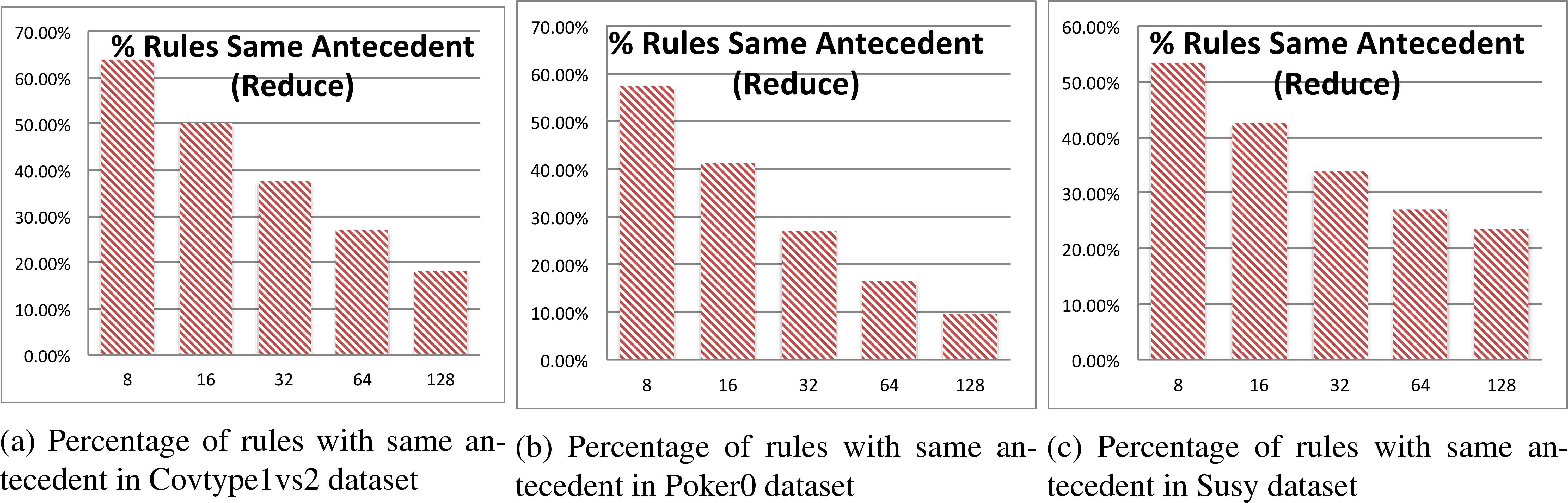
Percentage of rules with the same antecedent fed to the Reduce task.
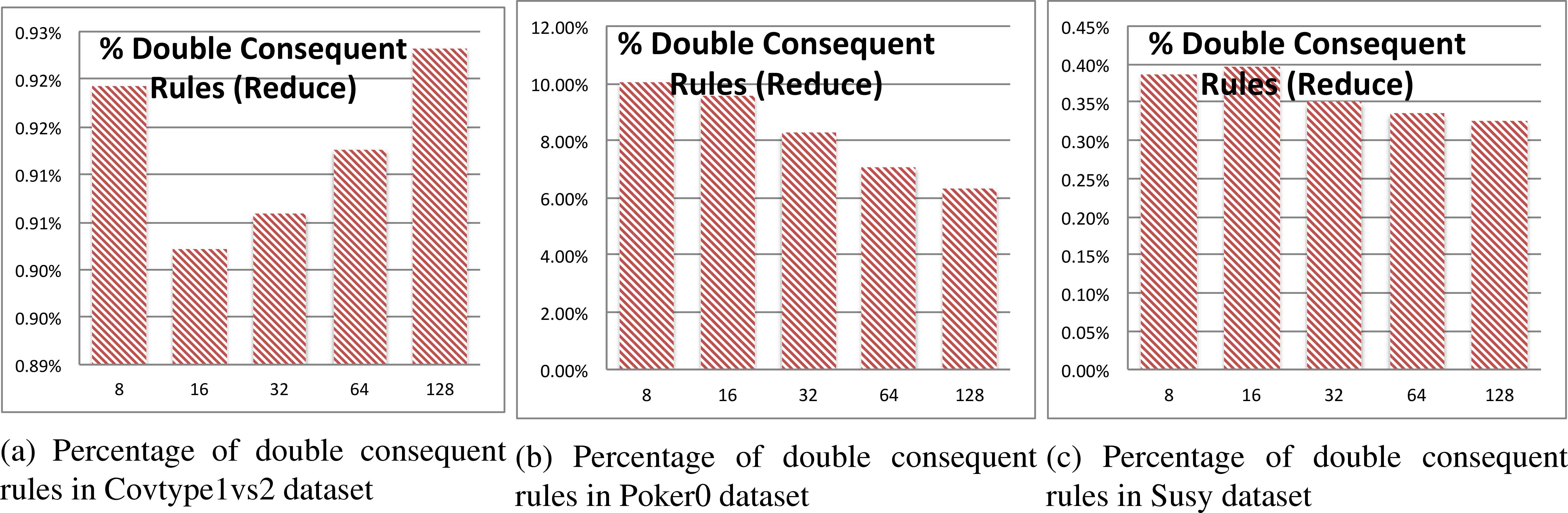
Percentage of rules with double consequent (same antecedent, different consequent).
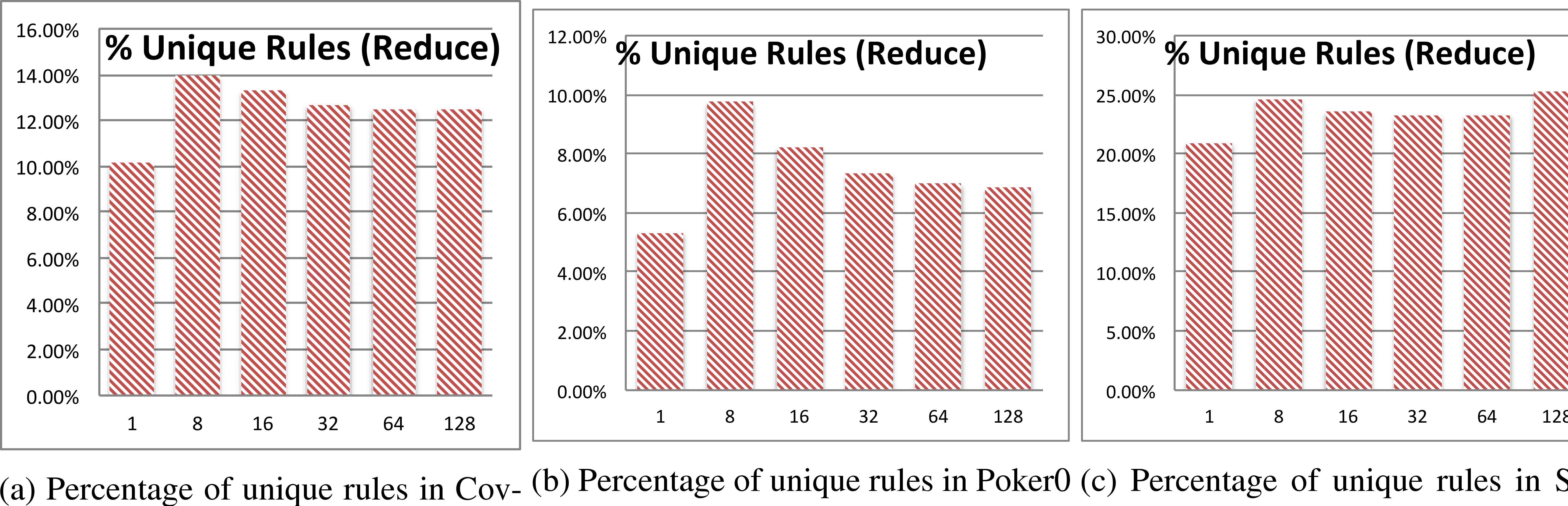
Percentage of rules discovered in a single Map over total.

Absolute number of rules discovered in a single Map over total.
5.2. Contribution of fuzzy rules to classification
Finally, we want to analyze the actual contribution of the different rules during the classification stage. To do so, we focus on the classification of the test partitions. Considering that we are applying the “winning rule” scheme, in which only the “strongest” rule is used to determine the class label, we may unequivocally compute how many rules from the total RB are selected for this purpose.
Results are illustrated in Figure 12. We divide the study into three parts, namely considering all rules without distinction (noted as “Total”), considering those rules whose antecedents have been mined along different maps (noted as [R > 1]]), and those rules that are generated on a single map (noted as [R = 1]). The percentages in each case are computed with respect to the number of rules of each type.
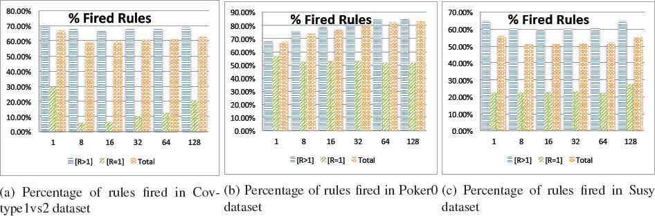
Percentage of rules fired in test classification according to their type.
First, we may conclude that in an FRBCS not all rules from the RB are finally used for classification. The reason is clear, as rules have a smooth overlapping among them, those in the core areas of a class cluster, i.e. with a high confidence and hence a high RW, will probably get a greater activation degree. Specifically, the average number of rules from total is about the 60% in all three case studies.
Additionally, there is a strong gap between those rules that are “repeated” along maps ([R > 1]) and “unique” rules ([R = 1), especially for Covtype1_vs_2 and Susy datasets. Rules discovered in several map tasks, will have associated a higher support, so that they are expected to cover a larger amount of instances.
Focusing on the behavior of “unique” rules, we must refer to the values shown in Figure 10 from Subsection 5.1. We conclude that the actual degree of contribution of this type of rules is low. From a percentage between the 10 and 20% of the total RB, just about a 10-30% are finally selected. However, these rules might be associated to examples from low density areas, thus being significant for the accurate representation of the whole problem space.
6. Lessons Learned and Discussion
In this paper, we have stressed the necessity of using novel computational paradigms to address Big Data problems. In particular, we have focused on the MapReduce programming framework due to its good properties for such a task. However, for standard MapReduce implementations, the workflow is initially divided into several processes, i.e. a local model is learned with a different chunk of the initial data. In this sense, we must take into account the ability of the baseline algorithms to carry out a robust local learning process.
Throughout our experimental study, we have investigated the capabilities of linguistic FRBCS to address this issue. The obtained results have shown that, even with few data, the fuzzy modeling is able to provide a good representation of the whole problem space, due to the coverage of the fuzzy labels.
This fact has several implications. The most straightforward one is the robustness of fuzzy models in case we need a higher scalability. Specifically, when a shorter elapsed time is required for the learning stage, the number of selected maps should be increased, leading to the problem of lack of data. However, we have shown that the accuracy of the individual / local fuzzy classifiers is somehow maintained even when using just about a 1% of the initial data. It has also been noted that when using more maps, local models become more similar among them. An additional strength of considering an homogeneous linguistic representation in MapReduce is related to the simplicity in the aggregation of the discovered rules. Finally, the fusion of these local RBs results on a global system with a higher quality.
However, this research arises several questions that must be addressed as future study.
The first one is related to the actual goodness of local learning and the limit or threshold for a good behavior. Concretely for fuzzy linguistic models, the main drawback is the computation of the RWs. As fewer data is considered for this task, these examples may be widely spread along the problem space and thus the RW will converge to 1.0. In case, it will be like RWs were not taken into account, and exactly the same number of rules will be obtained disregard the number of maps selected. However, there will be no straightforward heuristic to determine the consequent class of the rules neither for the local models, nor for the final aggregation.
The former point is also connected to whether RWs are actually necessary in Big Data applications. Traditionally, RWs have allowed FRBCS to have a better contextualization for the problem to solve, namely by considering these confidence degrees for guiding the inference process. However, not only RWs may become not significant when using a high number of maps, but their computation is actually a costly stage as examples must be iterated twice.
Considering all these must, the use of global fuzzy learning models must be analyzed 8. This type of approaches consider a core driver procedure to compile the partial results that are obtained by successive iterations of the algorithm. In spite the efficiency of global models is possibly slower, one may take advantage when implementing them withing a Spark environment 18.
The benefits and disadvantages of both local and global learning approaches must be carefully studied. Specifically, due to the good behavior shown by fuzzy local models, the use of more sophisticated fusion methodologies at the reduce stage may provide a leap of quality.
Another topic for further work is the dependence on the granularity level selected for the fuzzy partitions19. The choice of a higher number of labels be provide a more accurate representation of the problem space. However, this may also cause a rule explosion that is unfeasible in the context of Big Data. Therefore, filtering techniques, and / or a hierarchical approach 20 may lead to better results.
The previous issue arises another question: are homogeneous linguistic labels suitable for the learning in Big Data or do we need to contextualize the representation? This is a very interesting topic to be analyzed in depth, as it comprises several perspectives. On the one hand, whether to carry out an a apriori learning of the DB via strong fuzzy partitions that are properly adapted to the density related to each attribute of the dataset 21,22. On the other hand, to carry out a post-processing stage for the tuning of the membership functions 23,24.
The choice probably depends on two issues. First, on the efficiency that we are seeking for the learning stage. Second, on the actual difficulty of the problem measured in terms of the overlapping among classes. Specifically, when facing a Big Data problem the proportion of examples within clusters is expected to be high. This implies that the higher the support of the rules composing the RB, the higher the expected accuracy. Specifically, in our experimental study we have contrasted that few rules may comprise the majority of hits. In other words, misclassifications of “rare” cases are likely to be overwhelmed by a large amount of “common” examples. However, if we are facing a problem with highly overlapped classes, and/or an imbalanced dataset, too general rules will probably cause a bias for some of the classes.
In summary, we must be aware of the huge possibilities and benefits from the use of fuzzy logic in Big Data 7. The advantages are mainly a better coverage of the problem with probably a lower number of rules, the goodness of every individual local model, and the design of exact algorithms for allowing an optimal scalability.
7. Concluding remarks
In this work, we have analyzed the behavior of linguistic FRBCS in the context of Big Data. This implies the learning stage to be embedded into a MapReduce scheme. As such, it is distributed among different subtasks, each one of them devoted for a disjunct subset of the global dataset.
Our main goal was to acknowledge the properties and capabilities that allow FRBCS to be accurate and scalable. To accomplish this objective, we have carried out an experimental study with several Big Data classification problems. Through this process, we were able to extract some interesting information about the components of the RB during the MapReduce learning process at different levels of scalability, i.e. the number of selected Maps.
Among different issues, we have observed the robustness of fuzzy models when addressing the problem of lack of data. This fact implied that local models learned in each Map task are of high quality, and thus their aggregation boosts the recognition ability of the FRBCS. We have also identified that there is a high degree of replicated rules along the maps, i.e. identical rules are discovered within different subsets of the original data. This fact provides additional support to the previous finding, that is, partial RBs are able to represent accurately a high percentage of the problem space. Finally, we have observed that those fuzzy rules that are obtained from more than a map contribute the most to the final classification. From all these results we have concluded that FRBCS are actually a good choice when addressing Big Data classification problems.
As future work, we aim at designing new learning methodologies for FRBCS in MapReduce considering the conclusions extracted in this work. In particular, we intend to follow some of the guidelines provided throughout this paper, such as studying the effect of RWs, or analyzing the behavior of a global approach versus a local one.
Acknowledgment
This work have been partially supported by the Spanish Ministry of Science and Technology under projects TIN2014-57251-P and TIN2015-68454-R.
References
Cite this article
TY  - JOUR
AU  - Alberto Fernández
AU  - Abdulrahman Altalhi
AU  - Saleh Alshomrani
AU  - Francisco Herrera
PY  - 2017
DA  - 2017/08/30
TI  - Why Linguistic Fuzzy Rule Based Classification Systems perform well in Big Data Applications?
JO  - International Journal of Computational Intelligence Systems
SP  - 1211
EP  - 1225
VL  - 10
IS  - 1
SN  - 1875-6883
UR  - https://doi.org/10.2991/ijcis.10.1.80
DO  - 10.2991/ijcis.10.1.80
ID  - Fernández2017
ER  -