
Invariant moments based convolutional neural networks for image analysis
- DOI
- 10.2991/ijcis.2017.10.1.62How to use a DOI?
- Keywords
- Zernike moments; convolution kernel; invariant moments; pattern recognition; hierarchical feature learning
- Abstract
The paper proposes a method using convolutional neural network to effectively evaluate the discrimination between face and non face patterns, gender classification using facial images and facial expression recognition. The novelty of the method lies in the utilization of the initial trainable convolution kernels coefficients derived from the zernike moments by varying the moment order. The performance of the proposed method was compared with the convolutional neural network architecture that used random kernels as initial training parameters. The multilevel configuration of zernike moments was significant in extracting the shape information suitable for hierarchical feature learning to carry out image analysis and classification. Furthermore the results showed an outstanding performance of zernike moment based kernels in terms of the computation time and classification accuracy.
- Copyright
- © 2017, the Authors. Published by Atlantis Press.
- Open Access
- This is an open access article under the CC BY-NC license (http://creativecommons.org/licences/by-nc/4.0/).
1. Introduction
The advancement in the fields of data mining, biometrics, machine vision, medical imaging has increased the interest towards the advancement of image analysis, pattern recognition and classification(PRC). PRC systems are intelligent and are concerned with the extraction of robust and proficient attributes/features to describe and represent the objects for recognition and classification tasks. The features must be invariant to translation, scale and rotation, and should be independent and uncorrelated. The extraction and selection of reliable features decides the ability of the system in discriminating the classes or categories. The prime concern in PRC related to vision science (images) is how to extract the attributes automatically from the images and what sort of description and representation allows the system to learn the features and carry out the process of classification. As a result , the PRC systems are prescribed with the feature extractor that derives the features from the images and feeds them to a trainable classifier. Though learning good feature is very challenging because of large intra class visual variation in images, the literature shows a vast set of methods using hand crafted features such as Bag of words[1], Genetic Algorithm[2], Independent Component Analysis[3], Principal Component Analysis[4][5], Gabor transform[6], Histogram of Oriented Gradients[7], Scale invariant feature transform[8], Local Binary Pattern[9], Local Directional Pattern[10], Discrete Cosine Transform[11], Hidden Markov Model[12], Fourier Descriptors[13], Haralick features[14] and Invariant moments[15]. Though these hand crafted features are effective in representing and describing the images, they fail in extracting significant information and also convey a little semantic information[16][17]. This limitation is overcome by using deep network methods with multiple layered architecture for learning the features. The features extracted and learned from the deep networks are more reliable and also provide more amount of semantic information. The most successful deep learning method is the Convolutional Neural Network (CNN), wherein the lower level layers derive simple features and feed them to the higher level layers through forward propagation to extract the detailed features by convolving the images with the filters. Thus the feature learning is hierarchical and these features are excellent in representing the images for image analysis and PRC problems.
The idea of CNN has been inspired by the work of Hubel and Wiesel [18] on the cat’s primary visual cortex which resembled the architecture of CNN with multiple layers. The first model was proposed and implemented by Fukushima[19] and was called neocognitron. This was applied for handwritten digit recognition which further inspired several works related to CNN, that include classification of high resolution images[20], human action recognition[21], modeling sentences[22], scene labeling [23], matching natural language sentences[24], speech recognition[25], hand gesture recognition[26] and face recognition[27].
These methods achieved a considerable amount of accuracy by choosing random kernels as initial parameters for convolution and the kernels are picked from the normal distribution, which are not hierarchical to suit the layered architecture of CNN. However Zernike Moments(ZM) belonging to the class of orthogonal moments are better shape descriptors, where the lower order moments represent the global shape characteristics of the image and higher order moments provide detailed or finer shape information of the image[28][29].Thus the ZM possess a pyramidical architecture, through which the filter kernels as initial parameters can be derived by varying the moment orders as applicable to the different layers of CNN to achieve hierarchical feature learning.
The proposed method employs kernels for various layers of CNN derived from the ZM by varying the order of the moments as required to achieve significant amount of accuracy at a faster convergence rate. The rest of the paper is organized as follows. Section 2 describes the CNN. Section 3 presents derivation of convolutional kernels using invariant ZM. The experimental results employing ZM based kernels in CNN for various applications are discussed in Section 4. Finally Section 5 concludes the paper.
2. Convoutional Neural Network(CNN)
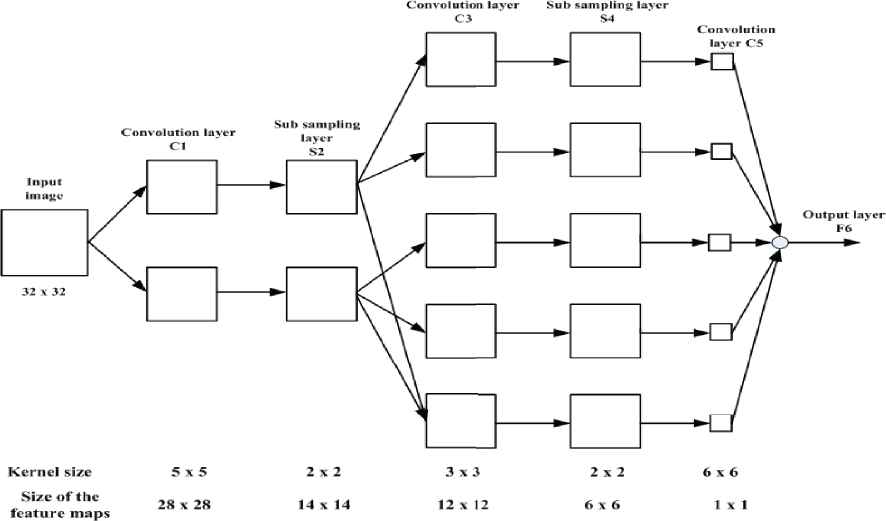
CNNs[30][31][32]are hierarchical deep neural networks with multistage architecture specially designed to process two dimensional data. The architecture is based on three key aspects: local receptive fields, weight sharing and sub sampling in the spatial domain. The strength of CNN lies in its features: - (a) Feature extraction and classification are integrated into structure and(b) It is invariant to translation and geometrical distortions in the images. Each stage of the architecture is composed of three layers: convolution layer, subsampling layer and nonlinear layer. Each convolution layer is followed by a subsampling layer and the last convolution layer is followed by an output layer or classification layer as shown in Fig.1. All the layers in CNN are 2D layers except the output layer which is one dimensional.
CNN network architecture
2.1 Convolution layer
Convolution layer is a 2D layer with several planes where each plane consists of neurons arranged in a 2D array. The output of each plane is called feature map. An output feature map is connected to the input feature map through a convolutional kernel, which is a matrix with trainable weights. Each plane computes convolution between its input and the kernel. Then the convolution outputs are summed and added with a trainable bias term. The output of the convolution layer is given by
- l
layer index
- *
convolution operator
-
feature map of the preceding layer
-
convolutional kernel from the feature map i in the preceding layer (l-1) to the feature map j of the layer l.
-
bias term associated with the feature map j.
-
list of all planes in layer (l-1) connected to the feature map j.
If size of the input feature map is H x Wand the size of the convolutional kernel is R x C, then the output feature map is of the size (H - R +1) x (W - C +1). Each plane in a convolution layer is connected to one or more feature maps of the preceding layer whereas each feature map is connected to one plane in the next subsampling layer.
Further each output map is multiplied by the connecting weights and added with a bias term which are trainable. The output of the subsampling layer is calculated as
-
matrix obtained after summing up or averaging each of the n x n blocks of the input feature map.
-
weight for the feature map j in sub sampling layer
-
bias term associated with the feature map j.
2.2 Subsampling layer
A subsampling layer down samples the input feature maps. The layer produces exactly the same amount of output feature maps as input feature maps. Here the input map is divided into distinct blocks of size n x n. These blocks are averaged or summed to produce an output which is n times smaller along both dimensions in the spatial domain. Thus the layer achieves spatial invariance to translation by reducing the size of the feature map.
If the size of the input feature map is H x W, then the size of the output map is (H/n x W/n). Each feature map of the subsampling layer is connected to one or more planes of the next convolution layer.
2.3 Nonlinear layer
It transforms the activation level of an unit into the output of pre determined range. Normally CNNs use the Pureline, Tan sigmoid , or Log sigmoid activation functions [33] in the nonlinear layer that follows convolution layer, subsampling layer of each stage, and the fully connected output layer.
2.4 Output layer
The output layer is fully connected to the convolution layer preceding it. It accepts the feature vector of an image from the previous layer and predicts the class label. The output of the layer is given by
- L
output layer index
- NL
number of neurons in the output layer
-
weight from feature map i of the last convolutional layer to jth neuron of the output layer
-
bias term associated with neuron j of layer L.
The outputs
2.5 Supervised learning of CNN
The supervised training of the CNN for image analysis and PRC requires assignment of the class labels to the training samples. During training, the training parameters such as the bias terms and the convolutional kernels associated with different layers of the network are modified to reduce the error function defined in terms of the desired outputs and actual outputs of the network. The error function is computed as shown
- K
number of input images
- NL
number of neurons in the output layer
- yk
kth actual output, which is a function of the bias terms and convolutional kernels
- dk
kth desired output
Thus, to achieve the reduction in error an appropriate training algorithm[30] has to be devised. These algorithms update the training parameters during learning according to the observed performance of the error function.
3. Zernike moments (ZM) based convolutional kernel
ZM[15][34] are projections of an image on to the complex zernike polynomials that are orthogonal over the unit circle. Zernike moment of order n and repetition factor m for a continuous image f(x, y) is defined as
Correspondingly the zernike moment of the digital image is obtained as shown,
-
normalization factor is the complex zernike polynomial given by
where,here Rnm(ρ) is the radial polynomial defined as
The ZM Anm are invariant to rotation, scale and translation. Due to the orthogonality and invariance properties, ZM make the best image descriptors and are very effective in deriving the shape characteristics [15][28][29]. These shape characteristics are very useful for image analysis and PRC problems. Further, the extraction of shape features rely on edge detection and hence the appropriate coefficients of the convolution kernel are to be estimated.
The convolution kernels of desired size are determined using the ZM as explained in [35]
- i.
Initially, based on the required size of the kernel an discrete image f(x, y)is assumed .
- ii.
For evaluating the ZM operator on image points, the proximity of the point should be mapped on to the interior of the unit circle as shown in Fig.2.
- iii.
After mapping, the coefficients of the kernel are obtained by evaluating the associated zernike moment integral over each pixel (Fig .2) assuming f(x, y) to be constant over that pixel using equation (9)for order n and repetition factor m. The kernel accordingly obtained for a dimension of 7x7 with n=4 and m=4 is shown in Fig 3.a.
- iv.
Finally, the kernel is to be convolved with an image to give the edge map. Fig 3.b and 3.c show an image and its edge detection based on zernike moments.
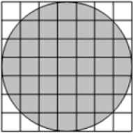
Mapping of f(x,y) with dimension 7x7 on to a unit circle
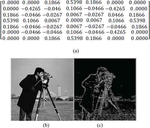
Convolutional kernel of size 7x7 obtained with n=4 and m=4 (a) Original cameraman image (b)and its edge detection(c) using 7x7 mask using (a)
3.1 CNN architecture adopted in this paper
To have more realistic comparison, the CNN architecture similar to that of [30] was employed for the proposed work as shown in Fig.1. The network consists of six layers. The input to the network is an image with dimension 32x32. The first layer C1 with two planes performs convolution on the input image using kernels of size 5x5 producing two feature maps of resolution 28 x 28 pixels. Then the sub sampling layer S2 down samples its input using window size of 2x2 to produce feature maps of size 14x14.This layer produces the same number of outputs as its inputs. Thus C1 and S2 have one to one connection as shown in Fig 1. Layer C3 is a convolutional layer that uses kernels of size 3x3 to produce five feature maps with each consisting of 12x12 pixels.
The connection between S2 and C3 is flexible and can be modified. The connection map is shown in Table 1.
| S2 | C3 |
||||
| x | x | o | o | x | |
| o | o | x | x | x | |
Connection map between S2 and C3
The Table 1 shows the connection between two feature maps of S2 and five feature maps of C3. A ‘x’ indicates the connection and ‘o’ indicates no connection. The subsampling layer S4 using a sampling window of size 2x2 produces five feature maps with size 6x6.The number of outputs and inputs of S4 are equal. C5 uses convolutional kernel of 6x6 to produce 6 scalar outputs for each of the input feature map. Thus the features for classification are available at the output of C5. Finally C5 is fully connected to the output layer F6 to produce a single network output.
The initial trainable convolutional kernels or masks for the layers C1,C3 and C5 were derived from ZM with variable order as explained in section 3.The convolutional layers present at different levels in the architecture extract features in a hierarchy. Accordingly, we used ZM as they have multilevel structure of extracting the features. The lower order moments present global shape patterns and the higher order moments present the detailed information of an image. Higher order moments are better shape descriptors and are sensitive to noise, so are to be selected carefully[29].
3.1.1 Convolution kernel selection
For the proposed work , a kernel set ‘K’ is initially formed from which the appropriate kernels to be assigned to the convolution layers are selected. This kernel set has range of kernels obtained by varying the ZM order from lowest to the highest. Each of the kernels present in K provide edge map based on the order of the moment. The edge map varies with the number of zero crossings and co-efficients in the zernike polynomial which in turn depends on the order and repetition factor of the polynomial. The lowest order selected is nmin=1 by ignoring the zeroth order as the corresponding zernike polynomial is flat over the unit circle and there exists no variance, hence does not convey any information. To select the highest order nmax image quality metric, peak signal to noise ratio(PSNR) is utilized. As the acceptable PSNR for an 8 bit gray level is 50dB[36], in our work, to have acceptable edge quality, the threshold was set at 60 dB .
A bench mark edge map was obtained using canny operator since it detects true edges with minimum error[37]. Four test images were considered for analysis :-lena, cameraman, flower and baboon. These images are chosen as they have sufficient number of gray levels and comprise of flat and detailed regions with shading and texture which make them able for testing and evaluation. The images along with their canny edge detection are shown in Fig 4.a and 4.b. Later, the ZM order and the corresponding repetition factor is varied from the lowest limit of nmin =1 to obtain the kernels and the corresponding edge maps of the test images to find the cumulative average PSNR, PSNRavg between the canny edge detected map and the edge maps obtained by the kernels. With each variation of n, the obtained PSNRavg is compared with PSNRmax. The value of n for which PSNRavg>PSNRmax is considered as nmax. For the test images considered, we have obtained nmax =18. As a result the kernel set with 91 kernels was obtained and is expressed as
- n
moment order
- m
repetition factor
- knm
convolutional kernel derived by varying n and m
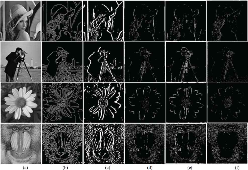
Original image(a) Edge detection using canny operator(b) k1,1 (c) k8,2(d) k14,10 (e) k18,2(f)
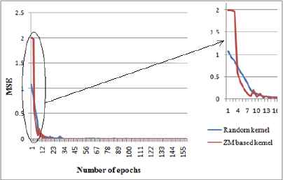
To select the appropriate kernels from K for CNN architecture, performance evaluation is initially carried out on K. For evaluation the bench marked edge maps obtained from the test images were used. For the same images the kernels from K were applied to get the edge maps. Few edge maps obtained using K are displayed in Figs 4.c - 4.f. From the edge maps it can be observed that lower order moments provide global shape characteristics and higher order moments represent the finer details of the image. Next, the metric mean square error (MSE) is computed between the canny edge detected map and the edge maps provided by all the kernels of K and Fig.5 shows the MSE obtained for the entire kernel set K with the four images. From the scatter plot, it can be noted that , the performance of the kernels is approximately the same for all the bench marked images.

MSE obtained between canny edge detected image and the edge images provided by the kernels from K
A lower valued MSE indicates the likeliness between the canny edge detected image and ZM based kernel edge detection indicating best performance in edge detection. Thus we choose the kernels that provide a smaller value of MSE from the kernel set. Accordingly a threshold value, MSEth = 0.03 was set. So, based on the selected threshold, the kernels that provided a MSE ≤ MSEth were selected. With this a new set K1 was framed with 46 kernels such that,
Later from K1 , the sum of the elements of each kernel Sk was computed as shown,
- knm
convolution kernel
- R x C
size of the kernel
- knm
convolution kernel
- R x C
size of the kernel
If Sk is zero it signifies that, kernel provides a better edge map by removing the constant part of the image. Hence from K1, the kernels that provided zero valued Sk were finally selected. The selected kernels thus formed K2 such that
Thus, based on the criterion explained above K2 has 22 number of kernels.
Finally, the kernels from K2 are to be assigned to layers C1,C3 and C5. Hence they are categorized into three groups (G1,G2 and G3) and from each group the kernels are selected randomly as initial parameters. The grouping is done in such a way that each kernel when selected at random gets an equal chance of being assigned to the convolution layer for training. The kernel assignment is illustrated in the Table 2.
| Group | G1 | G2 | G3 | |||||||
| Layer assignment | C1 | C3 | C5 | |||||||
| Order(n) | 1 | 2 | 4 | 6 | 8 | 10 | 12 | 14 | 16 | 18 |
| knm with order n and repetition m | k1,1 | k2,2 | k4,2 | k6,2 k6,6 | k8,2 k8,6 | k10,2 k10,6 k10,10 | k12,2 k12,6 k12,10 | k14,2 k14,4 k14,6 k14,10 | k16,2 k16,6 k16,10 k16,14 | k18,2 |
Division of selected kernels into three groups for convolutional layer assignment
From Table 2, G1 has 5 kernels, G2 has 8 kernels and G3 has 9 kernels. During the process of training the CNN, the kernels from the designated groups G1, G2 and G3 are randomly selected as initial parameters. According to the CNN architecture adopted in this paper, the layer C1 provides two feature maps, C3 five feature map and C5 five feature maps. Besides, each kernel when selected should get equal chance of getting trained. Thus two kernels when selected out of five from G1 get 40% chance in getting trained. Similarly five out of eight and five out of nine kernels when selected randomly from G2 and G3 respectively indicates 60% and 50% chance of getting trained . Also we can see that with this technique of categorization and assignment , on an average the kernels from each group gets an equal possibility of training to learn the features in hierarchy.
3. Results and Discussion
In the proposed method, ZM based kernels are chosen as initial trainable filters(CNN-ZM) for CNN. To evaluate the effectiveness of the method in hierarchical feature learning and thereby reducing the computation time to achieve faster convergence rate and accuracy, two discrete experiments were carried out using few image databases. Also the performance of the proposed method is compared with the architecture that uses random kernels(CNN-R) as initial parameters.
4.1 Experiment 1
The aim of the first experiment is to find the best discrimination between face and non face image patterns and classify gender using facial images based on CNN-ZM and CNN-R. To have a more realistic performance comparison between the proposed method and CNN-R, the CNN architecture similar to the one proposed in[30] was employed in our work.
4.1.1 Face and non face classification
The dataset for classification was extracted from ORL[38] and Face & skin detection database[39]. From ORL database 400 face images were taken and 400 non face images were considered from Face and skin detection database. Few samples of the dataset are depicted in Fig.6.a and 6.b. From the 800 images of the dataset 60% was used for training and the remaining 40% was used for testing. The training dataset is labeled for supervised learning and given as input to CNN which was described in section 2. The CNN is trained with back propagation algorithm which is a first order optimization method that tries to achieve the performance goal(Mean square error defined by equation (4)) of zero[30]. The evaluation was carried out under two cases
case (i): The initial bias terms for all the layers and convolutional kernels for C1, C3 and C5 are randomly selected from the normal distribution(CNN-R).
case(ii):The initial bias parameters are selected randomly from the normal distribution and convolutional kernels are selected from the respective groups formed using zernike moments. From these groups the kernels are selected randomly(CNN-ZM).
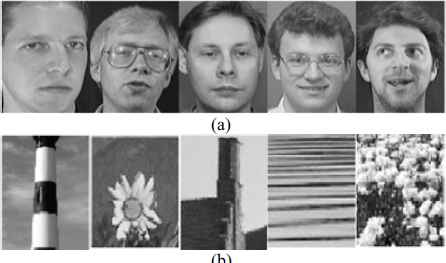
Sample images of face images (a) from ORL and non face images (b) from face and skin detection databases
Thus under both the cases, totally 316 parameters are trained by setting 1000 epoch limit. During training, the convolutional layers extract the edge information, subsampling layers reduce the size of the feature map and the non linear layers normalize the feature maps. Hence all the parameters are modified layer wise to learn the features in hierarchy. The CNN with the proposed method is iteratively trained and tested 10 times and also the convergence of the network under each iteration is noted. Both the methods converged to meet the required MSE. The performance of the system is evaluated using the metric accuracy. The classification results of ten iterations indicate that CNN-ZM was notable in reducing the computation time to attain faster convergence.
Though CNN-R was prominent in achieving the higher accuracy of 100% equal to that of CNN-ZM, computationally it was slower in reducing the function MSE. From the results it is also clear that CNN-ZM provided its best performance with 159 epochs whereas CNN-R converged with 221 epochs. The same is displayed in Fig.7.
Best performance curve for face and non face classification
The output of each layer for the best performance is displayed in Fig.8.a and 8.b. Also the output of last convolution layer is scalar quantity, hence it is not shown in the figures. From the figures it is seen that with the ZM based kernels, the edge information is significantly extracted in hierarchy providing the complete shape information as compared to random kernels.
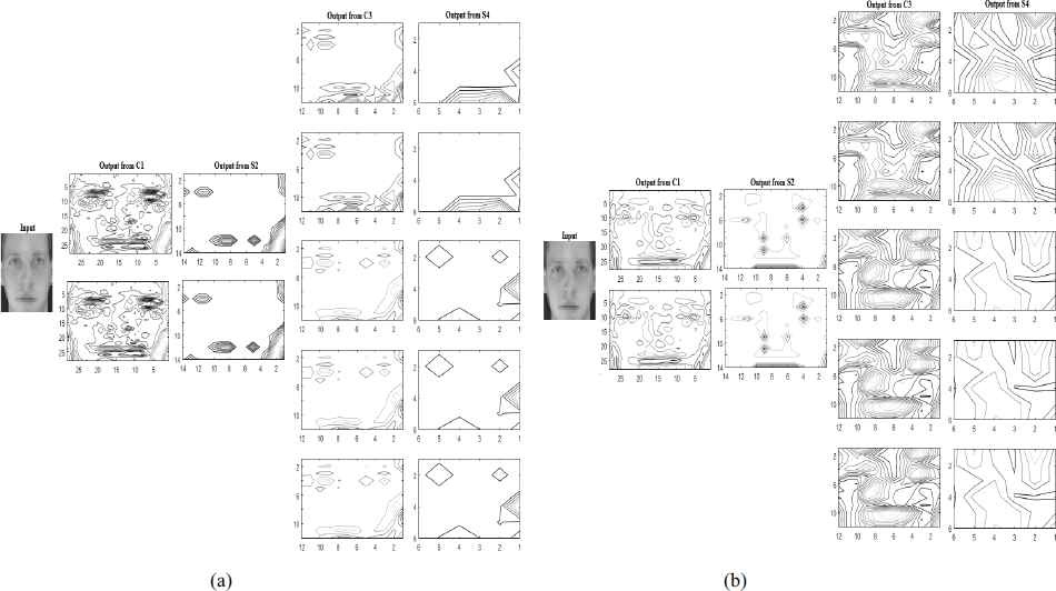
Output of each layer employing CNN-R(a) and CNN-ZM(b) for face and non face classification
4.1.2 Gender classification
Gender classification was carried out using faces94 database[40]. From the database 760 images of 38 subjects with different age groups and 20 images per subject were considered. Of 38 subjects, 19 are females and remaining 19 are males. Few of these images are with occlusion that include glasses and beard. Few samples of the dataset are displayed in Fig.9.a and 9.b.The dataset was divided into training and testing sets for feature learning, classification and evaluation. The process of gender recognition and classification was carried out in a similar way as followed in section 4.1.1. As mentioned earlier the CNN was iteratively trained for 10 times The classification results are shown in Table.3
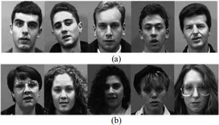
Sample images of male subjects (a) and female subjects from faces94 database
| CNN based on random kernels(CNN-R) | CNN based on ZM kernels(CNN-ZM) | |||||
|---|---|---|---|---|---|---|
|
|
||||||
| Iterations | Number of training epochs | Classification accuracy | MSE | Number of training epochs | Classification accuracy | MSE |
| 1 | 1000 | 94.74 | 0.053 | 597 | 95.79 | 0.0 |
| 2 | 1000 | 76.31 | 0.764 | 553 | 100 | 0.0 |
| 3 | 1000 | 57.37 | 0.776 | 652 | 100 | 0.0 |
| 4 | 1000 | 94.74 | 0.119 | 525 | 100 | 0.0 |
| 5 | 847 | 97.37 | 0.0 | 594 | 99.47 | 0.0 |
| 6 | 1000 | 78.42 | 0.566 | 552 | 98.42 | 0.0 |
| 7 | 702 | 96.85 | 0.0 | 544 | 99.47 | 0.0 |
| 8 | 992 | 98.42 | 0.0 | 474 | 100 | 0.0 |
| 9 | 863 | 92.64 | 0.0 | 776 | 95.27 | 0.0 |
| 10 | 639 | 98.95 | 0.0 | 669 | 98.95 | 0.0 |
Results for gender classification
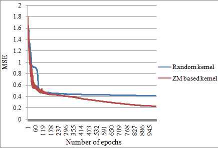
From Table.3 we see that the performance of CNNZM is very efficient in achieving the performance goal with faster convergence rate. Also the accuracy attained is higher as compared to CNN-R. The best performance of CNN-ZM was obtained at 474 epochs whereas CNN-R obtained at 639 epochs. The plot of the best performance is shown in Fig.10.Also the output of each layer for the best performance is displayed in Fig.11.a and 11.b, which illustrates the extraction of edges using CNN-ZM. Furthermore our method is significant in recognizing the gender of a person even with the presence of occlusions in the image.
Best performance curve for gender classification
Output of each layer ,employing CNN-R(a) and CNN-ZM (b)for gender classification
4.2 Experiment 2
The second experiment is intended towards recognizing the emotion of a person for which JAFFE database[41] was used. The database has 213 Japanese female images with seven different emotions of ten individuals. The emotions include angry, disgust, fear, happy, neutral, sad and surprise. Few sample images of the database are shown from Fig.12.
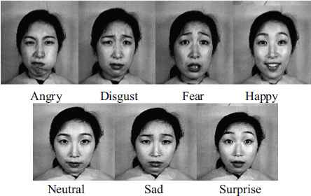
Sample images from JAFFE database indicating different emotions of an individual.
The work utilized the CNN architecture as that of [30], but with minor alteration where the connections between C5 and F6 are modified to get seven network outputs from F6 layer. This variation was done to map with the seven emotions that need to be recognized. The methodology of the work followed the same process that is explained in section 4.1. The facial expression recognition results are shown in Table.4
| CNN based on random kernels(CNN-R) | CNN based on ZM kernels(CNN-ZM) | |||||
|---|---|---|---|---|---|---|
|
|
||||||
| Iterations | Number of training epochs | Classification accuracy | MSE | Number of training epochs | Classification accuracy | MSE |
| 1 | 1000 | 85.33 | 0.4530 | 1000 | 85.53 | 0.2674 |
| 2 | 1000 | 83.08 | 0.3429 | 1000 | 83.08 | 0.1370 |
| 3 | 1000 | 85.53 | 0.4892 | 1000 | 87.60 | 0.2262 |
| 4 | 1000 | 85.53 | 0.4543 | 1000 | 83.65 | 0.2822 |
| 5 | 1000 | 84.40 | 0.444 | 1000 | 84.77 | 0.4028 |
| 6 | 1000 | 84.40 | 0.4345 | 1000 | 87.22 | 0.2602 |
| 7 | 1000 | 84.58 | 0.3805 | 1000 | 85.71 | 0.4898 |
| 8 | 1000 | 85.15 | 0.4505 | 1000 | 86.28 | 0.3027 |
| 9 | 1000 | 85.71 | 0.4152 | 1000 | 87.03 | 0.1124 |
| 10 | 1000 | 84.96 | 0.4454 | 1000 | 83.46 | 0.2134 |
Results for facial expression recognition
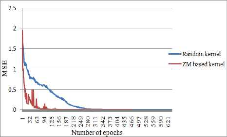
The classification results show that, CNN-ZM provided outstanding performance in recognizing the emotion of a person. The proposed CNN architecture was efficient in achieving the performance goal with fewer number of training epochs that signifies a faster convergence rate as illustrated in Fig.13.
Best performance curve for facial expression recognition
We can observe that CNN-ZM presented best performance of 87.6% for all the emotions where as CNN-R achieved 85.71% . From Table.4, it can also be noticed that when both CNN-ZM and CNN-R attained the same recognition accuracy, CNN-ZM was better with less MSE.
The recognition accuracy of individual emotions under the best performance condition is portrayed in Fig.14.
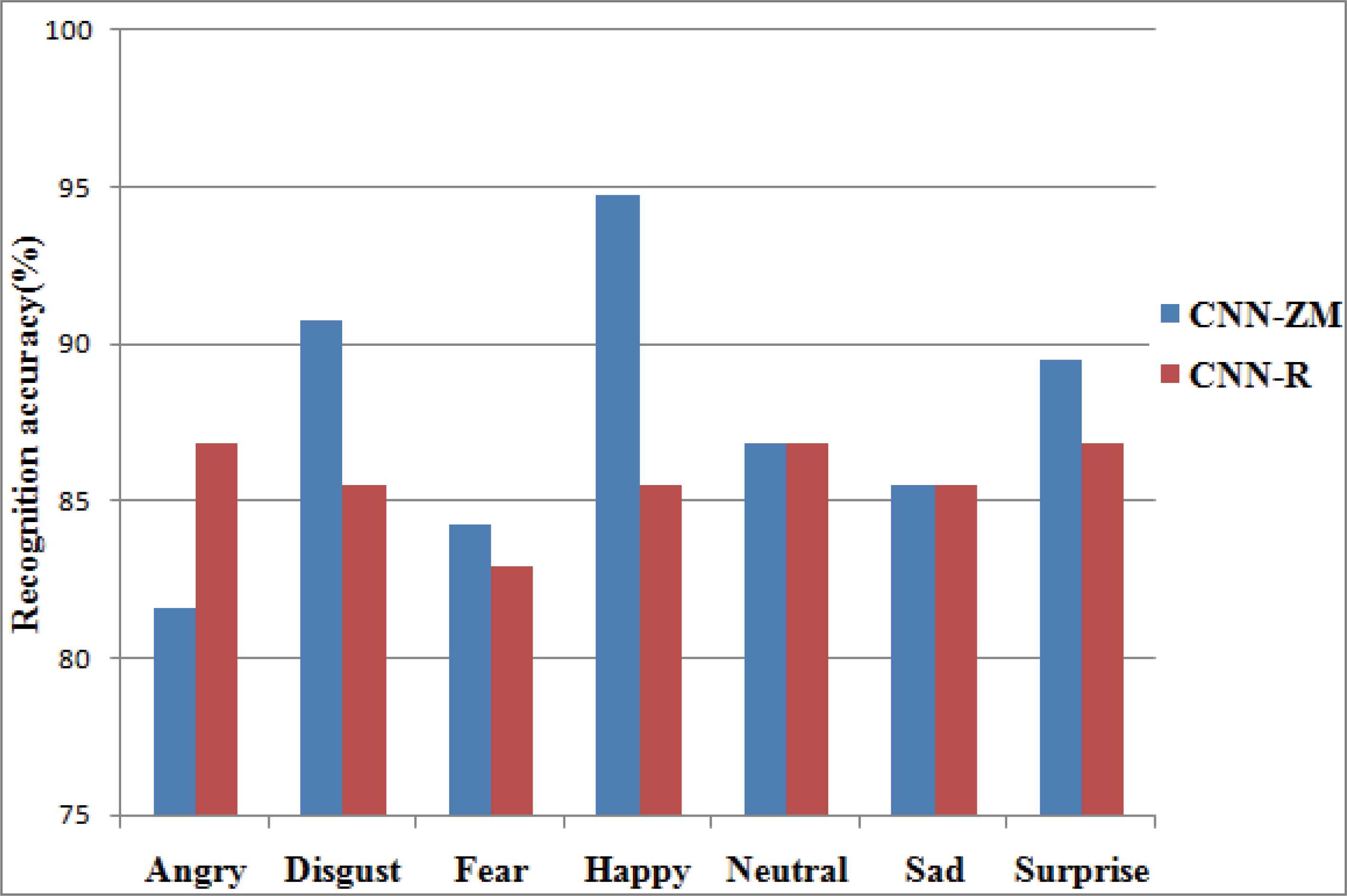
Recognition accuracy of individual emotions under the best performance
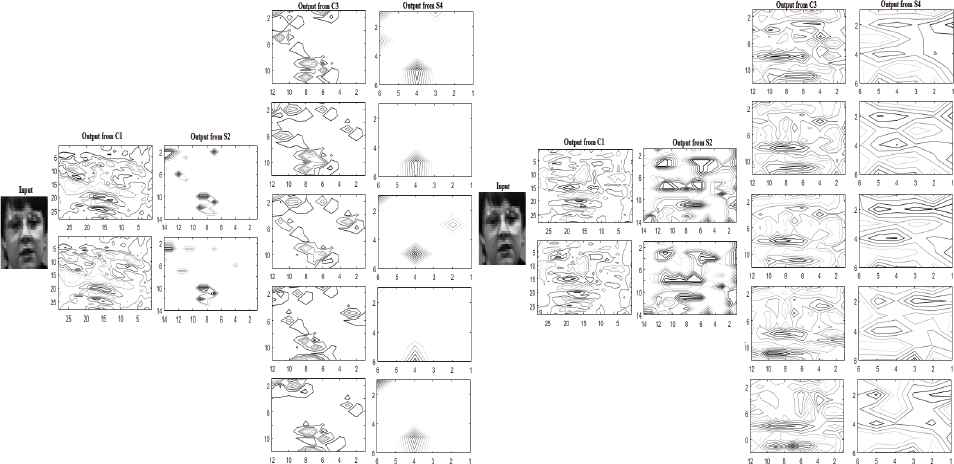
It can be observed that CNN-ZM has provided highest recognition accuracy of 90.79%, 84.21%, 94.74% and 89.5% for the emotions disgust, fear, happy and surprise respectively as compared to CNN-R with accuracy of 85.53%, 82.9%, 85.53% and 86.84%. The best edge detection is shown in Fig.15.a and 15.b using the contour plots of the detected edges at each stage.
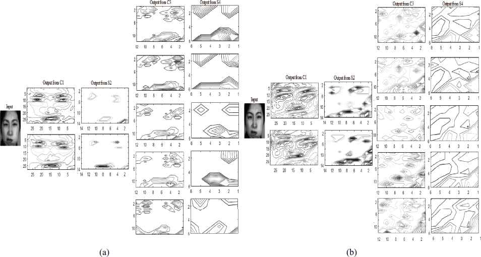
Output of each layer of employing (b) CNN-R and (b)CNN-ZM(b) for facial expression recognition
Finally, a concise comparison is made with our method and other approaches provided by different researchers for gender classification and facial expression recognition. But it is difficult to make an accurate comparison as a range of feature extraction methods are combined with different classifiers to achieve the task. The comparison is provided in Table.5. From the comparison it is found that the proposed work is comparable with other methods and is better in case of gender classification.
| Gender classification | Facial expression recognition | ||||||
|---|---|---|---|---|---|---|---|
| Methods | Database | Accuracy(%) | Computation time | Methods | Database | Accuracy(%) | Computation time |
| Topographic Independent Component Analysis+SVM[42] | Essex Face 94 + randomly collected images by Google search | 96 | - | ZM[46] | YALE JAFFE | 57.5 80.0 |
- |
| ZM with Fuzzy Inference system[43] | FERET | 85.05 | - | Facial landmarks+Gab or filter [47] | Moving Faces and People(MFP) | 63.74 (Average) |
- |
| CNN[44] | Adience | 86.8 | 10000 epochs | Gabor filter[48] | JAFFE Cohn-Kanade (CK) | 89.67 91.51 |
300 epochs 300 epochs |
| Gradient-LBP+SVM used on combination of both depth and gray scale images[45] | EURECOM Kinect Face dataset Texas 3D FR database | 94.23 95.30 |
- | Geometric features with SVM kNN[49] | Extended Cohn-kanade BU-4DFE | 73.63 67.17 68.04 57.92 |
- |
| Proposed method CNN-R [Convential CNN approach] CNN-ZM [Proposed approach] | Faces94 | 89(Average) 98.7(Average) |
904epochs (Average) 594epochs (Average) |
Proposed method CNN-R CNN-ZM | JAFFE | 84.8(Average) 85.4(Average) |
1000 epochs (Average) 1000epochs (Average) |
Comparative results of classification accuracy with other methods
4. Conclusion
In this work we presented a convolutional neural network for hierarchical feature learning and classification, where the trainable kernels for convolution layers were initialized using the parameters derived from zernike moments .The order of the zernike moments was varied from n=1 to n=18 and the suitable kernels were chosen based on performance evaluation carried out with respect to canny edge detection. The zernike moments with their multilevel structure are significant in providing both global and detailed shape characteristics of an image that made them suitable to be employed in CNN architecture.
The success of the proposed method was evaluated by testing it on ORL, face and skin detection, faces94 and JAFFE databases to carry out the tasks: face and non face classification, gender classification and facial expression recognition respectively.
The performance of the proposed method was also compared with the CNN architecture that was initialized using random kernels. Our method was excellent in extracting the edge information and also the results presented in Tables 3 and 4 indicated the remarkable performance of the zernike moment based kernels in achieving the predetermined goal(MSE=0) with lesser computation time indicating faster convergence rate as compared to random kernels. Additionally the classification accuracy obtained was comparable with the state of the art methods.
References
Cite this article
TY  - JOUR
AU  - Vijayalakshmi G.V. Mahesh
AU  - Alex Noel Joseph Raj
AU  - Zhun Fan
PY  - 2017
DA  - 2017/01/01
TI  - Invariant moments based convolutional neural networks for image analysis
JO  - International Journal of Computational Intelligence Systems
SP  - 936
EP  - 950
VL  - 10
IS  - 1
SN  - 1875-6883
UR  - https://doi.org/10.2991/ijcis.2017.10.1.62
DO  - 10.2991/ijcis.2017.10.1.62
ID  - Mahesh2017
ER  -