
GAB-BBO: Adaptive Biogeography Based Feature Selection Approach for Intrusion Detection
- DOI
- 10.2991/ijcis.2017.10.1.61How to use a DOI?
- Keywords
- NP-hard combinatorial optimization problem; biogeography based optimization; evolutionary state estimation approach; Hamming distance; Feature selection; intrusion detection
- Abstract
Feature selection is used as a preprocessing step in the resolution of many problems using machine learning. It aims to improve the classification accuracy, speed up the model generation process, reduce the model complexity and reduce the required storage space. Feature selection is an NP-hard combinatorial optimization problem. It is the process of selecting a subset of relevant, non-redundant features from the original ones. Among the works that are proposed to solve this problem, few are dedicated for intrusion detection. This paper presents a new feature selection approach for intrusion detection, using the Biogeography Based Optimization (BBO) algorithm. The approach which is named Guided Adaptive Binary Biogeography Based Optimization (GAB-BBO) uses the evolutionary state estimation (ESE) approach and a new migration and mutation operators. The ESE approach we propose in this paper uses the Hamming distance between the binary solutions to calculate an evolutionary factor f which determines the population diversity. During this process, fuzzy logic is used through a fuzzy classification method, to perform the transition between the numerical f value and four evolutionary states which are : convergence, exploration, exploitation and jumping out. According to the state identified, GAB-BBO adapts the algorithm behavior using a new adaptive strategy. The performances of GAB-BBO are evaluated on benchmark functions and the Kdd’99 intrusion detection dataset. In addition, we use other different datasets for further validation. Comparative study with other algorithms is performed and the results show the effectiveness of the proposed approach.
- Copyright
- © 2017, the Authors. Published by Atlantis Press.
- Open Access
- This is an open access article under the CC BY-NC license (http://creativecommons.org/licences/by-nc/4.0/).
1. Introduction
With the rapid progress in computer technologies, the traditional intrusion prevention systems alone such as firewall, encryption, antivirus software and secure network protocols, etc. have failed to provide robust protection against increasingly sophisticated attacks. Intrusion detection systems (IDS) are a second wall of defense where the events taking place in networks or computer systems are analyzed to detect whether they constitute normal activities or potential threats. Building an IDS relies on the following main steps: data collection, data preprocessing, intrusion detection and response 1.
Recently, machine learning techniques 2 are widely used to build effective IDS. The learning task uses a training data to induce a model which describes normal or attacks behaviors. When the model is generated, it can classify raw data into the corresponding classes (normal or a specific type of attack). The presence of irrelevant and redundant features in raw data may confuse the classifier leading to the deterioration of the detection performance. For this reason, Dimensionality Reduction (DR) has become a necessary step to go through before the actual training process. It aims to improve the classification accuracy, speed up the model generation process, reduce the model complexity and reduce the required storage space. DR is performed by Feature Extraction (FE) or Feature Selection (FS). FE is the process of generating a set of new features from the original ones (more compact and discriminant than the original ones). FS is the process of removing irrelevant and redundant features from the original ones. In contrast to FE, FS maintains the original features which is more useful for applications needing model interpreting and knowledge extraction 3. In intrusion detection, the semantic of the features is important for subsequent diagnosis of the cause of the attacks. In order to preserve the model interpretability and to improve the accuracy, we have opted in this work for feature selection.
Feature selection problem 3 is an active area of research in machine learning that has attracted a lot of attention. It is the process of selecting a subset of d relevant, non-redundant features from D original ones (d < D). FS consists in two important steps: subset search and subset evaluation. In the subset search step, candidate feature subsets are selected for the evaluation. In the subset evaluation step, the quality of the selected feature subsets is measured. According to the evaluation function, FS is mainly categorized in three categories: wrapper, filter and embedded approaches. A wrapper approach uses a learning algorithm to measure the learning performance obtained by each one of the generated feature subsets. The approach gives better accuracy. However, it is computationally expensive. A filter approach uses intrinsic characteristics of the training data to define an evaluation function. The evaluation function is used to evaluate each candidate feature subset instead of a learning algorithm. The filter approach is faster but less accurate than the wrapper approach. An Embedded approach performs feature selection within the learning algorithm. That is, the final result is a predictive model generated using a subset of features. The embedded approach is accurate and fast. However, the feature selection process it performs is not a separated step that can be combined with any learning algorithm (lack of flexibility). In this work, we have opted for the wrapper approach because of its accuracy and its flexibility. It is true that the wrapper approach suffers from its high computational cost. However, the time consumed by the FS algorithm does not affect the response time in the intrusion detection (feature selection is a preprocessing step which is not included in the intrusion detection process).Furthermore, the wrapper approach is considered very easy to parallelize, which will cope with the issue of the computation speed 4.
Finding the optimal feature subset is an NP-hard combinatorial optimization problem 4 with 2D − 2 subsets to explore. Therefore, for large-sized problem, the use of heuristics methods is required. In the wrapper FS problem providing a balance between exploration and exploitation is highly needed to find promising areas of the search space. To reach this balance, the use of adaptive metaheuristics is worthwhile. Biogeography Based Optimization (BBO) algorithm 5 is a powerful metaheuristic successfully applied in many applications 6. It offers a primitive adaptation mechanism which is improved in the approach proposed in this paper through a dynamic behavior adaptation leading to improvement of the exploitation and exploration balance. For all these reasons, BBO seems to be a good approach for the wrapper FS problem.
In this paper, we propose a new wrapper FS method using BBO. The proposed method which is named Guided Adaptive Binary Biogeography Based Optimization (GAB-BBO) uses new migration and mutation operators. Furthermore, it uses a modified Evolutionary State Estimation (ESE) approach to dynamically adapt the algorithm behavior. The idea of using ESE approach 7 to improve BBO algorithm has, best to our knowledge, not yet explored. The ESE approach analyzes the population diversity so as to identify the evolutionary states of the algorithm. Four evolutionary states (exploration, exploitation, convergence and jumping out) are defined based on an evolutionary factor f. The mapping between the numerical f value and the aforementioned evolutionary states is performed using fuzzy logic 8. The four different states are viewed as linguistic variables and the degree of membership of the f values in each one of these states is given by a specific membership function. According to the identified evolutionary state, GAB-BBO adapts the behavior of the algorithm. The algorithm parameters are dynamically adjusted to improve the exploration and the convergence abilities. Also, a Weighted Local Search (WLS) is used to improve the exploitation ability.
The rest of this paper is structured as follows: section 2 presents an overview of the existing feature selection methods. Section 3 is dedicated to an overview of BBO. Section 4 explains the proposed approach. Section 5 presents the experimental results. Finally, conclusion is given in section 6.
2. Overview of Feature Selection Methods
Feature selection is a necessary preprocessing step in many machine learning applications. It is an NP-hard combinatorial optimization problem 4. For large-sized problem, the exhaustive search of all subsets is computationally impractical which makes the use of heuristics methods unavoidable.
Most recently, population-based algorithms such as Genetic Algorithm (GA), Particle Swarm Optimization (PSO) and Ant Colony Optimization (ACO) have been used to solve the feature selection problem. Forsati et al.9 proposed a new version of ACO which was named Enriched Ant Colony Optimization (EACO) and applied it to the feature selection problem. The main idea in EACO is to embed the edges that were previously traversed in the earlier executions. Moayedikia et al.10 introduced a weighted bee colony optimization for the feature selection (FS-wBCO). The authors used global and local weights to measure the importance of the features and also a new recruiter selection procedure. Khushaba et al.11 proposed a Differential Evolution (DE) based feature selection algorithm. The generated feature subsets had a predefined size. A roulette wheel weighting scheme and a statistical repair mechanism were used to replace the duplicated features in the feature subsets. Al-Ani et al.12 also used the DE algorithm for the feature selection. Here all features were distributed in a set of wheels to improve the exploration ability. Unlike the population-based methods mentioned above, BBO algorithm was not widely used in the feature selection problem. Earlier version of BBO based feature selection was introduced by Yazdani et al.13. The authors proposed two versions with different solution encoding (binary and integer) and modified operators.
In intrusion detection more attention is given to feature extraction and classification and less research works have been proposed to solve the feature selection problem14. Among these works, we can mention the work of Gao et al.15 where ACO algorithm and SVM classifier were combined to find the most discriminative features in intrusion detection dataset. In the work of Eesa et al.16 a new algorithm named CuttleFish (CFA) was applied to the FS problem.
3. Overview of Biogeography Based Optimization (BBO)
BBO algorithm was introduced by Dan Simon in 2008 5. It was inspired by studies on the geographical distribution of biological species. Species can migrate between islands which are called habitats each of which represents a geographical area where species can live. The quality of life in each habitat is determined by a Habitat Suitability Index (HSI). Habitats that are suitable to the residence of species have a high HSI. The habitability is determined by the Suitability Index Variables (SIV). There are many factors in the real world which make a habitat more suitable to reside than others like rainfall, crop diversity, diversity of terrain, etc. Habitats with high HSI tend to have high number of species with high emigration rate and low immigration rate because they are saturated with species, while those with low HSI tend to have fewer species with low emigration rate and high immigration rate. In BBO metaheuristic, Dan Simon uses the following analogy:
- •
A habitat is analogous to a solution.
- •
A set of habitats is analogous to a population of solutions and the SIV describes the component of the solution.
- •
The HSI is analogous to the solution quality. Good solutions have high HSI and bad solutions have low HSI.
- •
The migration of species between habitats is analogous to the process of sharing SIV of good solutions with bad ones to improve their quality. This mechanism is called migration and it is of two types: immigration and emigration. For each habitat (Hi), in each iteration, the immigration rate λ and emigration rate μ are dynamically updated based on the fitness of the habitat as given in Eqs. (1) and (2)
where I and E are a user-defined maximum rates of immigration and emigration, respectively, N is the number of habitats in the population and K(i) is the rank of the ith habitat (Hi) according to its fitness (all habitats are sorted based on the fitness from the worst fitness to the best one). Good habitats have high value of μ and low value of λ. Thus, they have high probability to share their SIV with others and low probability to accept SIV from them. On the other hand, poor habitats have low value of μ and high value of λ. Thus, they have high probability to replace their SIV with others and low probability to share them. - •
The suddenly change in the SIV of the habitats, because of some occurring events like natural catastrophes, disease, etc., is analogous to the SIV mutation mechanism. The mutation aims to increase the exploration ability of the algorithm. It replaces the SIV of a selected habitat Hi by a randomly generated one. This mutation is performed according to a mutation rate mi given in Eq. (3).
where Mmax is a user-defined maximum mutation probability, Pi is the probability of having a rank k(i) and Pmax = Pj where j=arg max Pi, i=1,…,n.
The pseudo-code for BBO is given in algorithm 1.
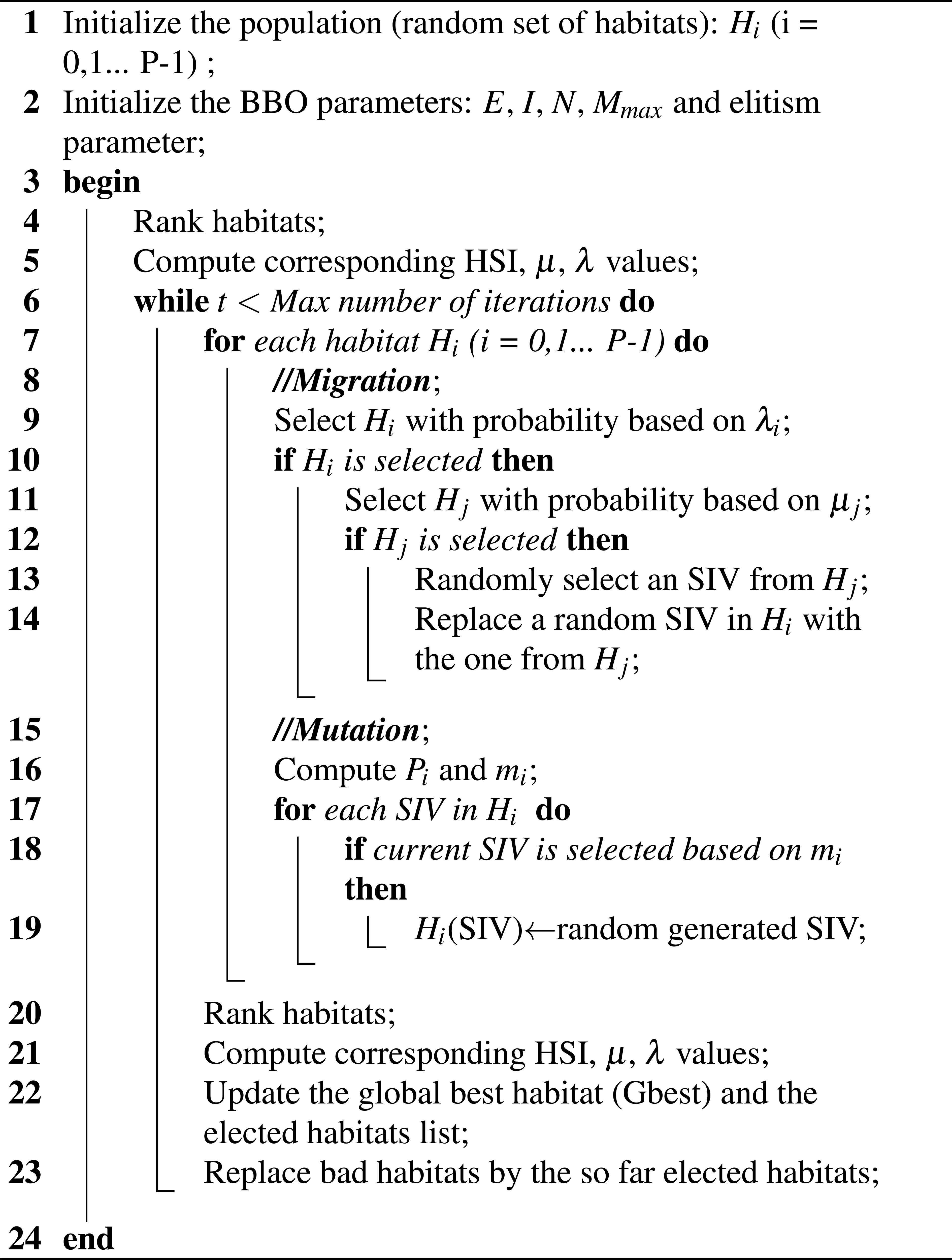
BBO.
4. Proposed Approach
The approach we propose which is named Guided Adaptive Binary Biogeography Based Optimization (GAB-BBO) is an improvement of the original BBO algorithm 5 applied to the feature selection problem. In the following subsections, we describe the main components of GAB-BBO. The general steps of this approach are depicted in algorithm 2.
4.1. Solution Representation
The solution for the feature selection problem is represented by a binary vector of dimension D, where each element is equal to 1 if the corresponding feature is selected and 0 otherwise (D being the total number of features).
In GAB-BBO algorithm, the search space is constituted by a set of habitats. Each habitat (Hi) corresponds to the binary vector with D SIV. Each SIV corresponds to a feature and has the values 1 (selected feature) or 0 (unselected feature). For example, Fig.1 describes a habitat with number of features D=10 where f3, f4 and f8 are the selected features. The total number of values equal to ’1’ in the binary vector corresponds to the number of selected features. In GAB-BBO this number is automatically determined and not fixed by a threshold value. Note that, in the sequel, solution and feature will refer to habitat and SIV, respectively.
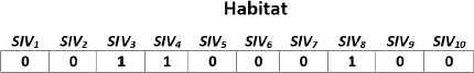
solution representation
4.2. Proposed Evolutionary State Estimation (ESE) Approach
In this paper, we propose to modify the ESE approach 7 and use it to dynamically adapt the behavior of the BBO algorithm. ESE approach analyzes the population distribution information so as to identify the evolutionary state of the algorithm. In each iteration, the mean Hamming distance between each solution and the rest ones is calculated to estimate one of the four evolutionary states namely: exploration, exploitation, convergence and jumping out. According to the identified state, an adaptive strategy is applied. We describe the details of the main steps of this process as follows:
Step 1: calculate the mean Hamming distance (di) between each habitat Hi and the rest ones as given in Eq. (4).
where N is the population size. In this equation, we propose to use the Hamming Distance (HD) instead of the Euclidean distance used in 7. HD between two binary vectors is the number of the different components.Step 2: determine the population diversity using an evolutionary factor f . To compute this factor, we first compare all the calculated distances (di), and then determine the maximal (dmax) and the minimal (dmin) distances. The evolutionary factor f is defined as given in Eq. (5).
where dg denotes di associated to the global best habitat.Step 3: classify the evolutionary factor f by a fuzzy classification method into one of the four evolutionary states: exploration, exploitation, convergence and jumping out. Fig. 2 shows the fuzzy set member ship functions used to classify f values.
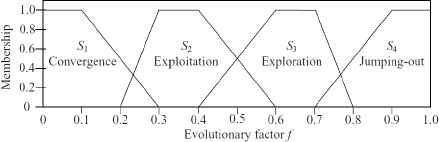 Fig. 2.
Fuzzy membership functions used to identify the different evolutionary states
The obtained f value is mapped into the membership functions which give the corresponding state. The small values of f (S1) describe the convergence state, the medium small values of f (S2) describe the exploitation state, the medium large values of f (S3) describe the exploration state and the large values of f (S4) describe the jumping out evolutionary state. To remove uncertainty when falling in overlapping regions, we use the following ideal sequence of states: exploration, then exploitation, then convergence, then jumping out.
Step 4: according to the evolutionary state identified, we apply new adaptive strategy. The treatments in each evolutionary state are defined as follows:
In the exploration state, we set Mmax parameter value to 0.9 (large value) so as to increase the mutation probability, leading thus to great exploration. Moreover, we set E and I parameters values to 0.2 (small value) so as to decrease the migration probability leading so to less exploitation. In this way, the algorithm searches in new regions.
In the exploitation state, we apply a Weighted Local Search (WLS) procedure to each habitat in the population so as to increase the exploitation ability of the algorithm.
In the convergence state, we decrease Mmax value to 0.1 and increase E and I values to 0.99. This will guide the habitats to the global best solution which allows a faster convergence.
In the jumping out state, we replace the current population by a new one that is randomly generated. This will jump the population toward a new region faster. We note that the adaptive strategy we presented above is mainly based on two treatments. The first one (parameter update) is used in the exploration and the convergence states whereas the second one (weighted local search) is used in the exploitation state. In what follows, we give some details about these two treatments.

GAB-BBO.
4.2.1. Parameter Update
Parameters E, I and Mmax influence widely the choice of the global or the local search in the search process. The idea behind the adaptive strategy is to dynamically modify these parameters according to the population distribution information, which is collected during each iteration, leading so to a dynamic behavior adaptation of GAB-BBO. Exploration is favored by high Mmax and low E,I values whereas convergence is favored by the reverse.
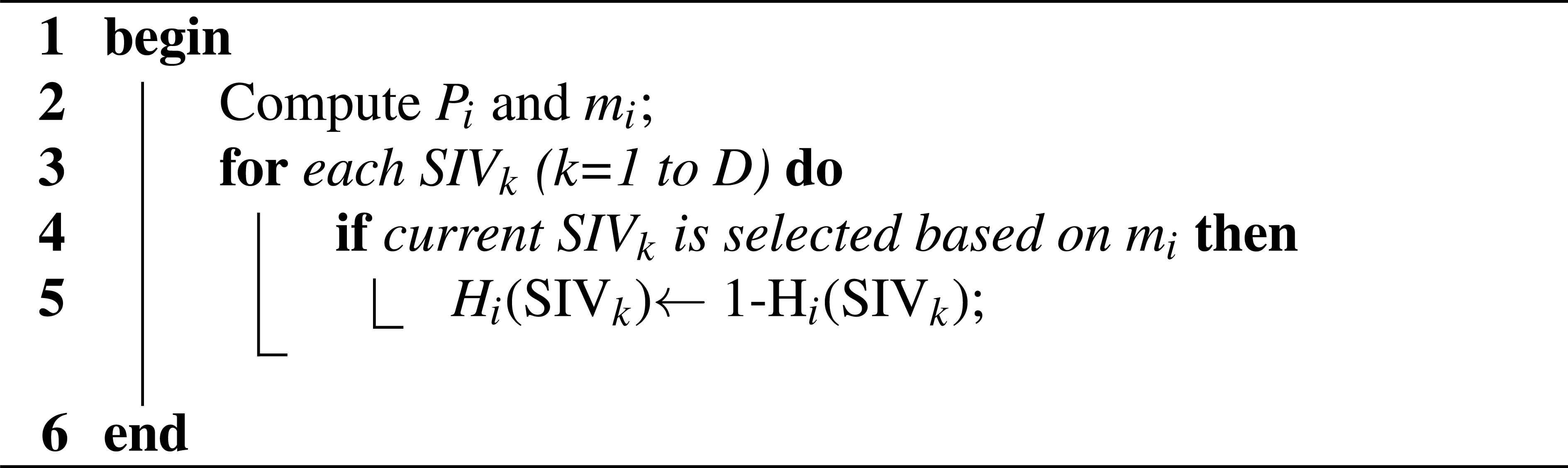
4.2.2. Weighted Local Search (WLS)
The proposed local search WLS attempts to enhance the quality of the habitat through the probabilistic transformation of SIV (features). We associate to each SIV a weight that measures its importance degree in the construction of good feature subsets. This means that SIV having a high importance degree contributes to produce better solutions. This weight is adaptively adjusted according to information which is collected during the search process. For each SIVk (k=1…D), the algorithm stores the following information :
- •
NbSelk is the total number of habitats that have SIVk =1 (selected feature).
- •
FitSelk is the summation of the fitness value of all habitats that have SIVk =1
- •
NbUnSelk is the total number of habitats that have SIVk =0 (unselected feature).
- •
FitUnSelk is the summation of the fitness value of all habitats that have SIVk =0
Using this information, WLS calculates the weight of each SIVk as given in Eq. (6) and the normalized weight as given in Eq. (7).

4.3. Proposed Binary Guided Migration
The general principal of the migration process in the original BBO algorithm is that good habitats (with high HSI) tend to share their SIV (features) with poor ones (with low HSI) so as to improve their quality. The immigration rate is used to probabilistically determine the poor habitat (Hi) that should modify its SIV and the emigration rate is used to probabilistically decide which of the good habitats should migrate their SIV to habitat Hi. The migration operator we propose is similar to this process. However, it differs in the way of accepting the new SIV that will replace the older one. We opt to replace an SIV by another one only if it improves the quality of the habitat. This process is described in algorithm 3.
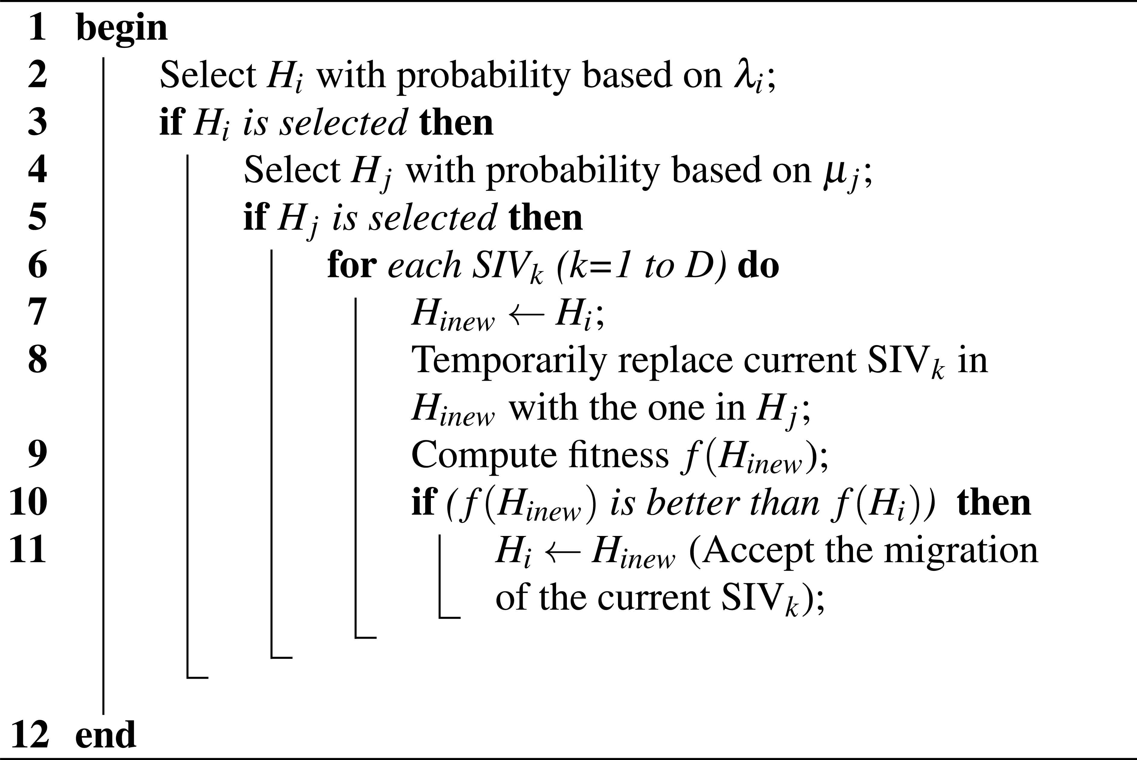
Binary Guided Migration.
4.4. Proposed Binary Mutation
Because we deal with binary coding scheme in which the SIV value can be either 1 or 0, we propose to modify the mutation of the original BBO. We use the binary mutation that is described in algorithm 4.
Binary mutation.
5. Experiments
To investigate the effectiveness of GAB-BBO, several experiments are carried out. In the following subsections, we firstly evaluate the performance of the proposed approach using 22 benchmark functions and compare it with other binary optimization algorithms. Then, we apply GAB-BBO to solve feature selection problem using intrusion detection dataset and compare its results with those of other feature selection methods. To further appreciate the performance of the proposed approach, we use other datasets in last experiments. Finally, we investigate the scalability. All experiments are conducted using Java 1.7 on workstation with 1.70 GHz Intel Core i5 4210U CPU and 8 GB main memory.
5.1. Performance Analysis Using the Benchmark Functions
The objective here is to analyze the convergence behavior of the GAB-BBO and compare its performance with other well-known binary optimization algorithms. All the results given in this section are from the average of 30 runs with 500 iterations and population of size 30.
5.1.1. Benchmark Functions
We use the benchmark functions introduced in the work of Mirjalili et al. 17 ( f1 to f22). These benchmark functions are categorized in three different groups: unimodal (f1 to f7), multimodal (f8 to f16) and composite functions (f17 to f22). Unimodal functions have only one global minimum solution and no local minimum solutions whereas multimodal functions have many local minimum solutions. Composite functions have also many local minimum solutions, however they have more complex structures and they are very similar to the fitness functions of real problems.
5.1.2. Convergence Behavior Analysis
To highlight the improvement of our algorithm in term of convergence, with respect to the original binary BBO, we compare the convergence speed of both algorithms.
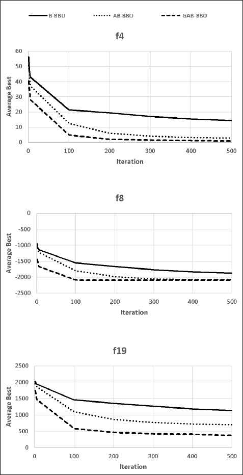
Fig.3 illustrates the averaged convergence curves for the unimodal function f4, the multimodal function f8 and the composite function f19. In these curves, we compare the convergence speed of the original binary BBO namely B-BBO 5, the proposed algorithm GAB-BBO and the algorithm namely ABBBO which is GAB-BBO algorithm without the proposed binary guided migration (we use instead the original migration operator).
averaged convergence curves of B-BBO, AB-BBO and GAB-BBO algorithms on some benchmark functions
Comparing GAB-BBO with AB-BBO aims to show the importance of the binary guided migration in the improvement of the convergence. Parameter values of B-BBO are fixed experimentally. Mmax is set to 0.9, E is set to 0.8 and I is set to 0.8. Parameter values of AB-BBO and GAB-BBO are dynamically adjusted using as initial values those of B-BBO.
According to Fig. 3, we observe that AB-BBO and GAB-BBO tend to converge faster than B-BBO for the selected functions. For the rest of the benchmark functions, experiments show that they remain converging faster than B-BBO. Therefore, we can conclude that the use of the ESE approach to dynamically adapt the algorithm behavior has widely improved the convergence speed. In addition, the proposed algorithm converges faster with the use of the binary guided migration.
5.1.3. Comparative Study
In this experiment, we compare the GAB-BBO approach with the Binary BBO (B-BBO) 5, the Binary Bat Algorithm (B-BA) 17, the Binary PSO (B-PSO) 17 and the Binary Genetic Algorithm (B-GA) 17 using the same precedent benchmark functions (f1 to f22).
In table 1, we present results of the comparison. These results are taken from the reference paper 17 and concern the average of the global best solution found in the last iteration. From table 1, we notice what follows:
By comparing GAB-BBO and B-BBO, we observe that the results obtained by GAB-BBO are widely better than those obtained by B-BBO for most of the benchmark functions. By comparing GAB-BBO, B-GA, B-PSO and B-BA, we observe that for all the unimodal and multimodal functions (except f14) GAB-BBO gives better results than the other algorithms. On the other hand, it gives better results than B-GA and B-PSO for all the composite functions whereas it gives better results than B-BA for the composite functions f17, f18 and f21. For f19, f20 and f22 B-BA performs better.
To statistically determine if the proposed algorithm gives a significant improvement over the aforesaid binary optimization algorithms, we perform the non-parametric Friedman test 18 using the Xlstat software. This statistical test ranks the different algorithms according to the average results of table 1. The statistic test results are shown in table 2. For a significance level alpha equal to 0.05, we found that the critical value is less than the observed value. Consequently, we can reject the null hypothesis which means that the difference between the algorithms is significant.
| B-GA | B-BA | B-PSO | B-BBO | GAB-BBO | fmin | |
|---|---|---|---|---|---|---|
| f1 | 10.0705 | 1.8518 | 5.2965 | 76.166664 | 0.0 | 0 |
| f2 | 0.2694 | 0.0965 | 0.2292 | 1.6333333 | 0.0 | 0 |
| f3 | 555.9039 | 7.8103 | 22.48915 | 232.3 | 0.0 | 0 |
| f4 | 1.59375 | 1.1526 | 2.6088 | 14.7 | 0.73333 | 0 |
| f5 | 369.7545 | 25.0743 | 148.0799 | 737.06665 | 1.6 | 0 |
| f6 | 6.9842 | 2.6993 | 8.4966 | 66.05 | 1.25 | 0 |
| f7 | 0.047174 | 0.0060 | 0.015542 | 0.0 | 0.0 | 0 |
| f8 | -929.324 | -985.320 | -988.355 | -1912.5645 | -2094.9138 | -418.9829 x 5 |
| f9 | 2.1896 | 1.5856 | 4.977688 | 0.6333333 | 0.0 | 0 |
| f10 | 1.399853 | 1.1560 | 2.725568 | 0.9396821 | 4.440892E-16 | 0 |
| f11 | 0.7067 | 0.2463 | 0.3873 | 1.8940364 | 0.0 | 0 |
| f12 | 0.191197 | 0.2708 | 0.621354 | 4.7307143 | 9.42327E-32 | 0 |
| f13 | 0.193006 | 0.1297 | 0.44445 | 1142.6733 | 1.3497843E-32 | 0 |
| f14 | -3.8849 | -3.6425 | -3.6416 | -1.5650622 | -1.5650684 | -4.687 |
| f15 | -0.474555 | -0.5173 | -0.055483 | -0.14559314 | -1.0 | -1 |
| f16 | 0.001575 | 3.198E-4 | 2.95E-4 | -1.0 | -1.0 | -1 |
| f17 | 193.6682 | 93.2475 | 194.8523 | 87.49375 | 13.522563 | 0 |
| f18 | 205.6785 | 156.6317 | 146.7613 | 166.41144 | 55.110798 | 0 |
| f19 | 384.7761 | 149.6407 | 445.7764 | 1135.6273 | 381.2022 | 0 |
| f20 | 588.1262 | 146.9480 | 479.9867 | 652.906 | 449.5591 | 0 |
| f21 | 246.3021 | 166.1212 | 172.0816 | 139.19975 | 44.124817 | 0 |
| f22 | 914.5375 | 152.8125 | 691.65 | 568.5127 | 457.36917 | 0 |
Minimization results of the Benchmark functions
| Results | GAB-BBO | B-BA | B-PSO | B-BBO | B-GA |
|---|---|---|---|---|---|
| Rank sum | 29 | 52 | 81 | 83 | 85 |
| Rank sum differences | - | 23 | 52 | 54 | 56 |
| Test results | α(significance level) = 0.05 | ||||
| df(degree of freedom)= k-1= 4 | |||||
|
|
|||||
|
|
|||||
| P-value < 0.0001 | |||||
| Rank sum Difference threshold = 20.556 | |||||
Ranks and test results for comparison of GAB-BBO with the used binary optimization algorithms
Furthermore, a pairwise comparison is performed to determine if the difference between our algorithm and the other algorithms is significant. The results indicate that the rank sum differences corresponding to each one of the algorithms B-BA, B-PSO, BBBO and B-GA are greater than the threshold value (20.556) which makes GAB-BBO significantly better than the other algorithms.
Based on the results obtained, GAB-BBO has proven to be a better option than the compared optimization procedures. It uses a dynamic behavior adaptation which does not exist in all the other algorithms but very important to guide the search process toward the best solution. Furthermore, B-BA, B-PSO, B-GA and B-BBO have too many parameters that highly affect the results. In GAB-BBO, the parameters are updated dynamically in the proposed adaptive behavior mechanism.
5.2. Application of GAB-BBO to Feature Selection Problem
In this section, the proposed approach is applied to solve the feature selection problem in intrusion detection field. We aim to select the most discriminative features that will contribute to improve the accuracy detection of the classifier. In this part of the work, we use Decision Tree (DT) as classifier 19 to measure the quality of each selected feature subset. DT is mainly characterized by being fast, simple, parameter-free and preventing overfiting.
To evaluate the proposed approach, we consider the Execution Time (ET), the number of selected features and the following classification performance measures:
- •
Detection Rate (DR) is the proportion of attacks that are correctly classified as attack.
- •
False Positive Rate (FPR) is the proportion of normal instances that are incorrectly classified as attacks.
- •
Accuracy Rate (AR) is the proportion of correctly classified instances.
- •
F-measure is a weighted average of precision and recall.
Where
5.2.1. Kdd’99 Dataset
In this experiment, we use the Kdd’99 dataset which is downloaded from http://kdd.ics.uci.edu. We choose Kdd’99 because it is the largest publicly available and the widest used dataset by the researchers in the intrusion detection field 16,14.
It contains a set of records (instances) describing TCP connections. The raw dataset consists of 41 features, 32 are continuous and 9 are discrete, and a label specifying the class. The class is labeled as either normal or attack with 24 types of attacks falling into four categories: Probe, Denial of Service (DoS), User to Root (U2R) and Remote to Local (R2L). Kdd’99 includes three independent sets: the whole Kdd training data with 4940000 records, 10% Kdd training data with 494021 records and Kdd test data with 311.028 records.
5.2.2. Experimental Steps
In this section, we describe the process of experiments consisting of four phases: data preprocessing, data reduction, training and testing.
- •
Data preprocessing phase consists of the following stages:
- •
Remove the redundancy records.
- •
Discretize the continuous features using Fayyad method 20. Discretization is performed to facilitate the computation of the correlation measure (correlation degree between each feature and the class label) used in one of the implemented algorithms, which is FS-wBCO.
- •
Remove two features (num outbound is_host_login) because their identical values in the 10% Kdd training data.
- •
Transform the Kdd’99 multiclass dataset to a binary one containing two classes: normal class and attack class.
- •
Divide the dataset into three independent parts: training subset, validation subset and test subset.
- •
Reduce the dataset size by applying a random subsampling method 21. A great deal of researchers in intrusion detection opt for sampling the Kdd99 dataset because it is a cumbersome dataset. We select randomly 6472 records from the 10% Kdd for the training subset, 1849 records and 925 records from the Kdd test data for the validation and the test subsets, respectively. The same proportion of instances in each class is kept as in the 10% Kdd training and Kdd test data. Table 3 gives the distribution of samples of each class in training, validation and test subsets.
Classes Training Validation Test Normal 2000 1159 581 attack 4472 690 344 Total 6472 1849 925 Table 3:Sample distribution on training, validation and test subsets
- •
- •
Data reduction phase uses the feature selection algorithm to select the best subset of relevant, non-redundant features. Since the proposed approach is of wrapper type, a classifier is used to evaluate the candidate feature subsets. The fitness function that is used in the proposed algorithm is the accuracy rate of the DT classifier on the validation subset.
- •
Training phase builds the model using the selected features.
- •
Testing phase evaluates the performance of the classifier on the test subset using the selected features. There are different ways to evaluate a learning process. Among them, cross validation and hold out evaluation methods. To evaluate our approach on the Kdd’99 dataset, we opt for the hold out evaluation because cross validation is computationally expensive.
5.2.3. Experimental Results and Comparisons
In this section, the GAB-BBO approach is evaluated and compared with other feature selection algorithms. The comparisons are divided into two parts. In the first part, we consider standard FS algorithms available in Weka 22 including filter algorithms (Information Gain (IG) 23, Gain Ratio (GR) 24 and Chi-Square (Chi-sq) 25), wrapper algorithms (Best First with Forward Selection (BF/FS) and best first with Backward Selection (BF/BS) 4) and embedded algorithms (SVM-FS 26 and OneR-FS 27). In the second part, GAB-BBO is compared with some implemented population-based FS algorithms which are FS-wBCO 10, RACOFS 9, DEFSw 12 and CBBBOFS 13. Parameters of these algorithms are experimentally fixed as shown in table 4.
| Algorithms | Parameter values |
|---|---|
| FS-wBCO | NC (number of constructive steps)=depends on the datasets size |
| RACOFS | γ(initial pheromone)=rand[0,1] α (concentration rate)=0.65 |
| DEFSw | Cr=0.5, F=0.4 |
| CBBBOFS | Mmax=0.9, E=0.8, I=0.8 |
Parameter values of the implemented algorithms
For the Kdd’99 dataset, the NC parameter (number of constructive steps in FS-wBCO) is set to 9. In order to perform a fair comparison, all population-based methods use the same number of iterations set to 50, the same population size set to 30 and the same initial solutions. All results obtained by the tested standard FS algorithms are from one run, because they are deterministic algorithms (give unique results). On the other hand, all results obtained by GAB-BBO and the implemented population-based FS algorithms are from average of 30 runs, because they are stochastic algorithms.
Note that, GAB-BBO, FS-wBCO and RACOFS have the ability to automatically determine the number of selected features. Thus, we retain the average value of all the found numbers over the 30 runs as number of selected features. On the other hand, DEFSw and CBBBOFS, need to have the number of features to select, as input parameter. Hence, we set it to the same number found by GAB-BBO.
Table 5 summarizes the results obtained by GAB-BBO and the standard FS algorithms. It presents, in the first line, the results obtained without any feature selection process.
| Methods | DR (%) | FPR (%) | AR (%) | F-measure | ET (s) | Number of selected features |
|---|---|---|---|---|---|---|
| All feature | 87.2 | 1.5 | 94.27 | 0.91 | - | All |
| GAB-BBO | 98.12 | 2.93 | 97.72 | 0.96 | 654.19 | 11 |
| IG | 87.5 | 1.9 | 94.16 | 0.91 | <1 | top11 |
| GR | 87.2 | 1.7 | 94.16 | 0.91 | <1 | top11 |
| Chi-sq | 87.5 | 1.9 | 94.16 | 0.91 | <1 | top11 |
| BF/FS | 91.3 | 2.6 | 95.13 | 0.93 | 4 | 4 |
| BF/BS | 87.8 | 1.9 | 94.26 | 0.91 | 52 | 11 |
| SVM-FS | 92.7 | 13.4 | 88.86 | 0.86 | 12 | top11 |
| OneR-FS | 87.8 | 1.7 | 94.37 | 0.92 | < 1 | top11 |
Comparisons of GAB-BBO with the standard FS algorithms on the kdd’99 dataset
The results indicate that the approach we proposed is able to reduce the dataset dimension by 71% (select 11 features from 39) improving substantially the performance in comparison to using all features. In addition, GAB-BBO is very competitive with respect to the standard FS algorithms in term of the classification performances. It gives DR equal to 98.12%, FPR equal to 2.93%, AR equal to 97.72% and F-measure equal to 0.96.
Table 6 presents the results given by GAB-BBO and the implemented population-based FS algorithms. The results indicate that GAB-BBO exhibits better classification performances with less or equal number of selected features.
| Methods | DR (%) | FPR (%) | AR (%) | F-measure | ET (s) | Number of selected features |
|---|---|---|---|---|---|---|
| GAB-BBO | 98.12 | 2.93 | 97.72 | 0.96 | 654.19 | 11 |
| DEFSw | 97.53 | 4.50 | 96.77 | 0.95 | 65.93 | 11 |
| CBBBOFS | 96.79 | 2.49 | 97.05 | 0.96 | 130.94 | 11 |
| RACOFS | 96.76 | 7.52 | 95.16 | 0.92 | 54.07 | 12 |
| FS-wBCO | 96.85 | 2.38 | 97.13 | 0.96 | 229.48 | 17 |
Comparisons of GAB-BBO with the implemented population-based FS algorithms on the kdd’99 dataset
In term of run time, GAB-BBO requires more time than the standard FS algorithms and than the implemented population-based FS algorithms. This time does not affect the detection response time, since feature selection is a preprocessing task that is not included in the intrusion detection process.
5.2.4. Validation Using Artificial Datasets
In this section, we evaluate our approach using artificial datasets 3 in which the optimal feature subset is known in advance. The total number of features, the number of instances and the relevant features of each selected dataset are given in table 7 .
| ID | Dataset | #feat. | # instances | Rel. feat. |
|---|---|---|---|---|
| CA | corrAl | 6 | 32 | 1-4 |
| CA100 | corrAl100 | 99 | 32 | 1-4 |
| M1 | Monk1 | 6 | 122 | 1,2,5 |
| M3 | Monk3 | 6 | 122 | 2,4,5 |
| P3 | Parity3+3 | 12 | 64 | 1-3 |
| L25 | Led25 | 24 | 50 | 1-7 |
| L100 | Led100 | 99 | 50 | 1-7 |
Details of the artificial datasets
The proposed approach is evaluated for each dataset and compared with the aforesaid feature selection algorithms. The evaluation is performed according to the Execution Time (ET), the average and maximum accuracy rate (Avg.AR and Max.AR) obtained in a 5-fold cross validation and the index of success (Succ.). Index of success (formula 14) is a scoring measure 3 that aims to reward the selection of relevant features and penalize the selection of redundant and irrelevant ones.
In table 8, we compare GAB-BBO with the standard FS algorithms. Results indicate that GAB-BBO gives similar or better accuracies than the standard FS algorithms. On CA dataset, GAB-BBO gives accuracy of 84.37% and selects all the relevant features. It performs similar to the wrapper algorithm BF/BS and better than BF/FS, the filter and the embedded algorithms. On CA100, GAB-BBO gives the best accuracy of 93.02% with index of success of 74% which is less than the one obtained by BF/BS. This is due to the fact that in CA100 dataset there are some irrelevant features that are informative to the classifier 3. On M1, the proposed algorithm gives accuracy of 100% and selects all the relevant features. These results are similar to those obtained by the wrapper methods and less than those obtained by the filter and the embedded methods. On M3, GAB-BBO gives the best index of success with accuracy of 93.44% which is similar to those obtained by all the standard FS methods. On P3, GABBBO achieves the best accuracy (100%) with best index of success (100%). These results are better than those obtained by all the standard FS methods. BF/BS reaches accuracy equal to 100% with index of success equal to -11%. This is due to the fact that BF/BS finds redundant features existing on P3 dataset 3 which leads to same accuracy than GABBBO (100%) with smallest index of success (-11%). On L25 and L100, the proposed method exhibits high accuracy and less index of success in comparison to the other standard algorithms. This is due to the noise which is included in the datasets and which assigns to the relevant features an incorrect values 3. Table 10 shows the Friedman statistic test of the maximum accuracy rate of table 8. The test results indicate that the null hypothesis is rejected (critical value is less than the observed value) which means that the difference between the algorithms is significant. Pairwise comparison shows that GAB-BBO is significantly better than the filter and the embedded FS algorithms. For the wrapper algorithms (BF/FS and BF/BS), GAB-BBO achieves similar results.
| Datasets | Measures | GAB-BBO | IG | GR | Chi-sq | BF/FS | BF/BS | SVM-FS | OneR-FS |
|---|---|---|---|---|---|---|---|---|---|
| CA | Avg.AR(%) | 84.37 | - | - | - | - | - | - | - |
| Max.AR(%) | 84.37 | 59.37 | 59.37 | 59.37 | 75 | 84.37 | 75 | 81.25 | |
| ET(s) | 13.39 | < 1 | < 1 | < 1 | < 1 | < 1 | < 1 | < 1 | |
| Rel.feat. | 1-4 | 2,3,4 | 2,3,4 | 2,3,4 | - | 1-4 | 1-4 | 1-4 | |
| #Irr.feat. | 0 | 2 | 2 | 2 | 1 | 0 | 1 | 1 | |
| Succ.(%) | 100 | 25 | 25 | 25 | -25 | 100 | 75 | 75 | |
| CA100 | Avg.AR(%) | 93.02 | - | - | - | - | - | - | - |
| Max.AR(%) | 93.75 | 53.12 | 53.12 | 53.12 | 84.37 | 90.62 | 53.12 | 59.37 | |
| ET(s) | 172.60 | < 1 | < 1 | < 1 | 2 | 96 | 1 | < 1 | |
| Rel.feat. | 1,2,4 | - | - | - | - | 1-4 | 4 | 1,3,4 | |
| #Irr.feat. | 12 | 10 | 10 | 10 | 3 | 6 | 9 | 7 | |
| Succ.(%) | 74 | -0.44 | -0.44 | -0.44 | -0.13 | 99 | 24 | 74 | |
| M1 | Avg.AR(%) | 100 | - | - | - | - | - | - | - |
| Max.AR(%) | 100 | 98.38 | 98.38 | 98.38 | 100 | 100 | 92.74 | 92.74 | |
| ET(s) | 24 | < 1 | < 1 | < 1 | < 1 | < 1 | < 1 | < 1 | |
| Rel.feat. | 1,2,5 | 1,2,5 | 1,2,5 | 1,2,5 | 1,2,5 | 1,2,5 | 1,2,5 | 1,2,5 | |
| #Irr.feat. | 0 | 2 | 2 | 2 | 0 | 0 | 2 | 2 | |
| Succ.(%) | 100 | 66 | 66 | 66 | 100 | 100 | 66 | 66 | |
| M3 | Avg.AR(%) | 93.44 | - | - | - | - | - | - | - |
| Max.AR(%) | 93.44 | 93.44 | 93.44 | 93.44 | 93.44 | 93.44 | 93.44 | 93.44 | |
| ET(s) | 20.50 | < 1 | < 1 | < 1 | < 1 | < 1 | < 1 | < 1 | |
| Rel.feat. | 2,4,5 | 2,4,5 | 2,4,5 | 2,4,5 | 2,5 | 2,5 | 2,4,5 | 2,4,5 | |
| #Irr.feat. | 1 | 2 | 2 | 2 | 0 | 0 | 2 | 2 | |
| Succ.(%) | 83 | 66 | 66 | 66 | 66 | 66 | 66 | 66 | |
| P3 | Avg.AR(%) | 100 | - | - | - | - | - | - | - |
| Max.AR(%) | 100 | 78.12 | 78.12 | 78.12 | 96.87 | 100 | 54.68 | 56.25 | |
| ET(s) | 20.55 | < 1 | < 1 | < 1 | < 1 | < 1 | < 1 | < 1 | |
| Rel.feat. | 1-3 | 2,3 | 2,3 | 2,3 | 1-3 | - | - | - | |
| #Irr.feat. | 0 | 3 | 3 | 3 | 4 | 3 | 5 | 5 | |
| Succ.(%) | 100 | 55 | 55 | 55 | 85 | -11 | -18 | -18 | |
| L25 | Avg.AR(%) | 57.33 | - | - | - | - | - | - | - |
| Max.AR(%) | 58 | 36 | 36 | 36 | 52 | 50 | 18 | 42 | |
| ET(s) | 51.47 | < 1 | < 1 | < 1 | 2 | 3 | 1 | < 1 | |
| Rel.feat. | 1,2,7 | 1-7 | 1-7 | 1-7 | 1,2 | 1,2 | 5,7 | 1-7 | |
| #Irr.feat. | 2 | 3 | 3 | 3 | 3 | 3 | 8 | 3 | |
| Succ.(%) | 38 | 92 | 92 | 92 | 21 | 21 | 9 | 92 | |
| L100 | Avg.AR(%) | 60.53 | - | - | - | - | - | - | - |
| Max.AR(%) | 64 | 38 | 40 | 38 | 60 | 54 | 34 | 42 | |
| ET(s) | 223.41 | < 1 | < 1 | < 1 | 4 | 142 | 9 | < 1 | |
| Rel.feat. | 1,2 | 1,2,4,5,7 | 1,2,4-7 | 1,2,4,5,7 | 1,2 | 1,2,5 | 5,7 | 1,2,5,7 | |
| #Irr.feat. | 4 | 5 | 4 | 1 | 2 | 8 | 6 | ||
| Succ.(%) | 28 | 71 | 85 | 71 | 28 | 42 | 27 | 56 |
Results of GAB-BBO and the standard FS algorithms on the artificial datasets
| Datasets | Measures | GAB-BBO | DEFSw | CBBBOFS | RACOFS | FS-wBCO |
|---|---|---|---|---|---|---|
| CA | Avg.AR(%) | 84.37 | 75.62 | 84.37 | 78.02 | 84.37 |
| Max.AR(%) | 84.37 | 84.37 | 84.37 | 78.12 | 84.37 | |
| ET(s) | 13.39 | 2.16 | 9.39 | 3.53 | 3.44 | |
| Rel.feat. | 1-4 | 1-4 | 1-4 | 1 | 1-4 | |
| #Irr.feat. | 0 | 0 | 0 | 2 | 0 | |
| Succ.(%) | 100 | 100 | 100 | -25 | 100 | |
| CA100 | Avg.AR(%) | 93.02 | 83.43 | 83.95 | 71.14 | 87.5 |
| Max.AR(%) | 93.75 | 90.62 | 87.5 | 78.12 | 87.5 | |
| ET(s) | 172.60 | 6.05 | 11.19 | 13.99 | 25.08 | |
| Rel.feat. | 1,2,4 | 2 | - | - | 1-4 | |
| #Irr.feat. | 12 | 3 | 4 | 6 | 5 | |
| Succ.(%) | 74 | 24 | -0.17 | -0.26 | 99 | |
| M1 | Avg.AR(%) | 100 | 93.99 | 100 | 88.11 | 100 |
| Max.AR(%) | 100 | 100 | 100 | 99.19 | 100 | |
| ET(s) | 24 | 9.13 | 12.81 | 6.89 | 33.62 | |
| Rel.feat. | 1,2,5 | 1,2,5 | 1,2,5 | 1,2,5 | 1,2,5 | |
| #Irr.feat. | 0 | 0 | 0 | 2 | 0 | |
| Succ.(%) | 100 | 100 | 100 | 66 | 100 | |
| M3 | Avg.AR(%) | 93.44 | 92.92 | 93.44 | 93.44 | 93.44 |
| Max.AR(%) | 93.44 | 93.44 | 93.44 | 93.44 | 93.44 | |
| ET(s) | 20.50 | 7.69 | 13.13 | 6.45 | 25.30 | |
| Rel.feat. | 2,4,5 | 2,4,5 | 2,5 | 2 | 2,5 | |
| #Irr.feat. | 1 | 0 | 1 | 1 | 1 | |
| Succ.(%) | 83 | 100 | 50 | 50 | 50 | |
| P3 | Avg.AR(%) | 100 | 96.92 | 100 | 70.41 | 100 |
| Max.AR(%) | 100 | 100 | 100 | 90.62 | 100 | |
| ET(s) | 20.55 | 5.18 | 9.66 | 6.04 | 12.91 | |
| Rel.feat. | 1-3 | 1,2 | 1-3 | 1-3 | 1-3 | |
| #Irr.feat. | 0 | 1 | 0 | 1 | 0 | |
| Succ.(%) | 100 | 62 | 100 | 96 | 100 | |
| L25 | Avg.AR(%) | 57.33 | 53.33 | 52.73 | 35.13 | 54.6 |
| Max.AR(%) | 58 | 56 | 58 | 40 | 56 | |
| ET(s) | 51.47 | 9.89 | 19.37 | 9.42 | 24.54 | |
| Rel.feat. | 1,2,7 | 1,2,5,6 | 1,2,7 | 1-7 | 1,2,5,7 | |
| #Irr.feat. | 2 | 3 | 4 | 7 | 0 | |
| Succ.(%) | 38 | 49 | 33 | 83 | 57 | |
| L100 | Avg.AR(%) | 60.53 | 59.33 | 47.86 | 29 | 49.6 |
| Max.AR(%) | 64 | 64 | 60 | 38 | 56 | |
| ET(s) | 223.41 | 10.58 | 20.65 | 19.20 | 56.99 | |
| Rel.feat. | 1,2 | 1,2,6 | 1,2 | 1,3,5,7 | 1,4,5 | |
| #Irr.feat. | 4 | 4 | 5 | 41 | 6 | |
| Succ.(%) | 28 | 42 | 28 | 53 | 42 |
Results of GAB-BBO and the implemented population-based FS algorithms on the artificial datasets
| Results | GAB-BBO | BF/BS | BF/FS | OneR-FS | GR | IG | Chi-sq | SVM-FS |
|---|---|---|---|---|---|---|---|---|
| Rank sum | 50.5 | 45.5 | 42 | 29 | 24 | 22.5 | 22.5 | 16 |
| Rank sum differences | - | 5 | 8.5 | 21.5 | 26.5 | 28 | 28 | 34.5 |
| Test results | α(significance level) = 0.05 | |||||||
| df(degree of freedom)= k-1=7 | ||||||||
|
|
||||||||
|
|
||||||||
| P-value < 0.0001 | ||||||||
| Rank sum Difference threshold = 17,96 | ||||||||
Ranks and test results for comparison of GAB-BBO with the standard FS algorithms on the artificial datasets
In table 9, we give the results obtained by GABBBO and the implemented population-based FS algorithms over the used artificial datasets. These results show that GAB-BBO performs better than DEFSw and RACOFS on most datasets. Furthermore, it performs better than CBBBOFS on L25 and L100 and better than FS-wBCO on CA100, L25 and L100. Friedman test results, which are presented in table 11, show that our algorithm is significantly better than DEFSw and RACOFS. For CBBBOFS and FS-wBCO, GAB-BBO gives similar results.
| Results | GAB-BBO | FS-wBCO | CBBBOFS | DEFSw | RACOFS |
|---|---|---|---|---|---|
| Rank sum | 30,5 | 26,5 | 22.5 | 15 | 10,5 |
| Rank sum differences | - | 4 | 8 | 15 | 20 |
| Test results | α(significance level) = 0.05 | ||||
| df(degree of freedom)= k-1=4 | |||||
|
|
|||||
|
|
|||||
| P-value =0.001 | |||||
| Rank sum Difference threshold = 11.595 | |||||
Ranks and test results for comparison of GAB-BBO with the population-based FS algorithms on the artificial datasets
Furthermore, we note in table 8 and 9 that GABBBO requires more execution time than all the standard and population-based FS algorithms. However, this time remains reasonable.
5.2.5. Validation Using Real-Problem Datasets
To further evaluate the effectiveness of the proposed approach, the same previous comparisons are performed using seven real-problem datasets with different number of features.
Table 12 presents the details of each selected dataset. The first column corresponds to the identifier of the datasets (ID). The second, third and fourth columns correspond to the description of the datasets. The fifth column corresponds to the number of samples in each portion of the datasets and the last column gives the NC parameter values.
| ID | Dataset | Number of feature | Number of instances | Training/validating/testing | NC |
|---|---|---|---|---|---|
| BC | Breast cancer | 9 | 699 | 489/139/71 | 3 |
| lO | Ionosphere | 35 | 351 | 246/70/35 | 9 |
| KR | Kr_Vs_Kp | 36 | 3196 | 2236/638/322 | 5 |
| SB | Spame base | 57 | 4601 | 3220/966/415 | 15 |
| HV | Hill Valley | 101 | 606 | 400/176/30 | 75 |
| MUS1 | MUSK 1 | 168 | 476 | 272/144/60 | 126 |
| LU | Lung | 325 | 73 | 51/14/8 | 243 |
Details of the real-problem datasets
The first six datasets are downloaded from http://archive.ics.uci.edu/ml/index.html and the last one from http://penglab.janelia.org/proj/mRMR/FAQ_mrmr.htm
The proposed approach is evaluated on each selected dataset and compared with the aforesaid FS algorithms. The comparison is based on the average Accuracy Rate (AR), Execution Time (ET) and the number of selected features.
In table 13, we compare the use of all features with GAB-BBO and the standard FS algorithms. The results show that GAB-BBO outperforms the standard FS algorithms and gives much better accuracies on all the datasets when compared with the results obtained using all features. On BC dataset, GAB-BBO gives the best accuracy of 95.77% with 5 features and among the standard algorithms, only wrapper algorithms (BF/FS and BF/BS) and the embedded algorithm OneR-FS are able to improve the performance with accuracy of 92.95%. On IO dataset, all the standard algorithms improve the accuracy, however GAB-BBO achieves much better accuracy of 97.14% with number of features equal to 16. On KR, SB and HV datasets, GAB-BBO remarkably improves the accuracy and no improvement can be achieved using the standard FS algorithms. Also on MUS1 and LU datasets, GAB-BBO gives the best accuracy of 84.5% with 79 features and 86.25% with 130 features, respectively.
| Datasets | Measures | All-features | GAB-BBO | IG | GR | Chi-sq | BF/FS | BF/BS | SVM-FS | OneR-FS |
|---|---|---|---|---|---|---|---|---|---|---|
| BC | AR(%) | 91.54 | 95.77 | 91.54 | 91.54 | 91.54 | 92.95 | 92.95 | 91.54 | 92.95 |
| ET(s) | 18.04 | < 1 | < 1 | < 1 | 1 | 1 | < 1 | < 1 | ||
| #feat. | 5 | top 5 | top 5 | top 5 | 7 | 6 | top 5 | top 5 | ||
| lO | AR(%) | 85.71 | 97.14 | 88.57 | 88.57 | 88.57 | 91.42 | 88.57 | 88.57 | 88.57 |
| ET(s) | 17.93 | < 1 | < 1 | < 1 | 2 | 2 | < 1 | < 1 | ||
| #feat. | 16 | top 16 | top 16 | top 16 | 7 | 8 | top16 | top16 | ||
| KR | AR(%) | 93.78 | 98.72 | 93.78 | 93.78 | 93.78 | 93.47 | 93.16 | 75.77 | 93.47 |
| ET(s) | 215.92 | < 1 | < 1 | < 1 | 2 | 17 | 1 | < 1 | ||
| #feat. | 22 | top 22 | top 22 | top 22 | 9 | 25 | top22 | top22 | ||
| SB | AR(%) | 83.85 | 89.18 | 82.40 | 80.48 | 79.27 | 82.89 | 77.59 | 87.71 | 69.63 |
| ET(s) | 1034.10 | < 1 | < 1 | < 1 | 29 | 205 | 8 | < 1 | ||
| #feat. | 17 | top 17 | top 17 | top 17 | 26 | 34 | top17 | top17 | ||
| HV | AR(%) | 53.33 | 61.33 | 53.33 | 53.33 | 53.33 | 50 | 50 | 53.33 | 53.33 |
| ET(s) | 131.08 | < 1 | < 1 | < 1 | 1 | 34 | < 1 | < 1 | ||
| #feat. | 39 | top 39 | top 39 | top 39 | 6 | 7 | top39 | top39 | ||
| MUS1 | AR(%) | 66.66 | 84.5 | 68.7 | 68.33 | 68.7 | 51.66 | 51.66 | 51.66 | 66.66 |
| ET(s) | 2633.45 | < 1 | < 1 | < 1 | 4 | 87 | 6 | < 1 | ||
| #feat. | 79 | top 79 | top 79 | top 79 | 10 | 10 | top79 | top79 | ||
| LU | AR(%) | 50 | 86.25 | 37.5 | 37.5 | 37.5 | 75 | 62.5 | 62.5 | 25 |
| ET(s) | 858.25 | 1 | 1 | 1 | 2 | 400 | 13 | < 1 | ||
| #feat. | 130 | top 130 | top 130 | top 130 | 6 | 9 | top130 | top130 |
Results of GAB-BBO and the standard FS algorithms on the real-problem datasets
To show whether the difference between algorithms is significant, Friedman test is performed. The test results, which are given in table 14, show that GABBBO is significantly better than all the standard FS algorithms.
| Results | GAB-BBO | BF/FS | IG | Chi-sq | GR | SVM-FS | OneR-FS | BF/BS |
|---|---|---|---|---|---|---|---|---|
| Rank sum | 56 | 33 | 31,5 | 29,5 | 29 | 26,5 | 24 | 22,5 |
| Rank sum differences | - | 23 | 24 | 26.5 | 27 | 29 | 32 | 33 |
| Test results | α(significance level) = 0.05 | |||||||
| df(degree of freedom)= k-1=7 | ||||||||
|
|
||||||||
|
|
||||||||
| P-value=0.003 | ||||||||
| Rank sum Difference threshold = 17,963 | ||||||||
Ranks and test results for comparison of GAB-BBO with the standard FS algorithms on the real-problem datasets
In table 15, the comparisons are made with the implemented population-based FS algorithms. Results indicate that GAB-BBO is competitive with respect to the other population-based FS algorithms in term of accuracy rate. On BC dataset, our algorithm gives the best accuracy with 95.77%. On IO dataset, the proposed algorithm is better than FS-wBCO and mostly better than DEFSw, CBBBOFS and RACOFS. On KR dataset, GAB-BBO achieves better accuracy than DEFSw, CBBBOFS and FS-wBCO and much better than RACOFS. On SB dataset, the proposed algorithm gives better accuracy than DEFSw and CBBBOFS and mostly better accuracy than RACOFS and FS-wBCO with reduced number of features. On HV and MUS1 datasets, GAB-BBO shows the best accuracy among all algorithms with 61.33% and 84.5%, respectively. On LU dataset, GAB-BBO gives similar accuracy than CBBBOFS and outperforms the other algorithms. Friedman statistic test results, which are given in table 16, show that the null hypothesis is rejected which means that the difference between the algorithms is significant. Pairwise comparison reveals that GAB-BBO is significantly better than DEFSw, FS-wBCO and RACOFS. For CBBBOFS, GAB-BBO shows similar performances.
| Datasets | Measure | GAB-BBO | DEFSw | CBBBOFS | RACOFS | FS-wBCO |
|---|---|---|---|---|---|---|
| BC | AR(%) | 95.77 | 95.16 | 95.07 | 94.03 | 94.36 |
| ET(s) | 18.04 | 5.66 | 12.10 | 4.19 | 13.13 | |
| #feat. | 5 | 5 | 5 | 4 | 4 | |
| lO | AR(%) | 97.14 | 94.38 | 95.42 | 92.09 | 96.85 |
| ET(s) | 17.93 | 3.24 | 5.36 | 4.41 | 9.23 | |
| #feat. | 16 | 16 | 16 | 8 | 12 | |
| KR | AR(%) | 98.72 | 97.14 | 97.63 | 91.27 | 97.73 |
| ET(s) | 215.92 | 51.35 | 83.39 | 13.04 | 16.28 | |
| #feat. | 22 | 22 | 22 | 24 | 22 | |
| SB | AR(%) | 89.18 | 88.36 | 87.87 | 84.62 | 85.95 |
| ET(s) | 1034.10 | 63.21 | 126.33 | 23.35 | 40.45 | |
| #feat. | 17 | 17 | 17 | 23 | 25 | |
| HV | AR(%) | 61.33 | 55.99 | 58.33 | 60 | 53.33 |
| ET(s) | 131.08 | 6.33 | 16.72 | 13.81 | 3.12 | |
| #feat. | 39 | 39 | 39 | 3 | 33 | |
| MUS1 | AR(%) | 84.5 | 81.16 | 83.66 | 81.16 | 82.49 |
| ET(s) | 2633.45 | 117.69 | 192.65 | 55.57 | 51.27 | |
| #feat. | 79 | 79 | 79 | 42 | 62 | |
| LU | AR(%) | 86.25 | 77.5 | 86.25 | 53.75 | 66.25 |
| ET(s) | 858.25 | 17.61 | 43.09 | 109.67 | 23.76 | |
| #feat. | 130 | 130 | 130 | 62 | 114 |
Results of GAB-BBO and the implemented population-based FS algorithms on the real problem datasets
| Results | GAB-BBO | CBBBOFS | DEFSw | FS-wBCO | RACOFS |
|---|---|---|---|---|---|
| Rank sum | 34,5 | 23,5 | 18,5 | 18 | 10,5 |
| Rank sum differences | - | 11 | 16 | 16.5 | 24 |
| Test results | α(significance level) = 0.05 | ||||
| df(degree of freedom)= k-1=4 | |||||
|
|
|||||
|
|
|||||
| P-value =0.001 | |||||
| Rank sum Difference threshold = 11.595 | |||||
Ranks and test results for comparison of GAB-BBO with the population-based FS algorithms on the real-problem datasets
In term of execution time, we remark from tables 13 and 15 that GAB-BBO is more time consuming than standard and population-based FS algorithms. This lack of computation speed is compensated by a gain in classification accuracy.
5.2.6. Approach Scalability
In this section, we analyze the scalability of GABBBO approach by calculating the execution time for different problem sizes. Fig. 4 illustrates the curve of the execution time evolution according to the problem size (dataset dimension ranging from 9 to 325 features). The estimated equation of this curve is polynomial of degree four which confirms the scalability of the proposed approach.

Evolution of the execution time according to the dimension
6. Conclusion
Feature selection is an NP-hard combinatorial optimization problem. It is the process of selecting a subset of relevant, non-redundant features from the original ones.
In this paper, we propose an improved version of the Biogeography Based Optimization (BBO) algorithm to solve the feature selection problem in intrusion detection. In the new approach, which is abbreviated as GAB-BBO, we propose to improve the original migration and mutation processes through a new binary guided migration and a new binary mutation, respectively. Furthermore, we modify the Evolutionary State Estimation (ESE) approach and use it to dynamically adapt the algorithm behavior. In the proposed ESE approach, we first use the Hamming distance between the binary solutions to calculate an evolutionary factor f. Then, we use the fuzzy logic to determine the evolutionary state of the algorithm from the obtained f value. According to the identified state, we adapt the algorithm behavior using new adaptive strategy based on parameter update and Weighted Local Search (WLS) procedure.
Two experiments have been conducted. In the first one, the performances of GAB-BBO have been evaluated using benchmark functions and compared with other binary optimization algorithms. In the second one, we have applied the proposed approach to solve the feature selection problem using the Kdd’99 intrusion detection dataset and compared it with other feature selection methods. The comparative studies show the competitiveness of GAB-BBO. For further validation, the same previous experiment has been performed using artificial and real-problem datasets confirming the effectiveness of the proposed approach. Finally, the approach scalability has been investigated through the study of the execution time evolution according to different problem sizes (number of features). The latter experiment shows the scalability of GAB-BBO. It has been concluded that the proposed approach constitutes a good solution for feature selection problem.
As future work, we plan to improve the execution time by proposing a distributed version of our algorithm. Also we plan to modify our algorithm for multi-class classification. To further improve the accuracy, we intend to hybrid the proposed algorithm with different local search strategies such as: simulated annealing, tabu search and variable neighborhood search. Finally, in the experiments, we will investigate alternative evaluation methods such as n folds cross validation with other classifiers such as ANN, KNN and SVM.
Acknowledgement
The authors would like to thank the associate editor and anonymous reviewers for their valuable comments that have significantly helped to improve the paper quality.
References
Cite this article
TY  - JOUR
AU  - Wassila Guendouzi
AU  - Abdelmadjid Boukra
PY  - 2017
DA  - 2017/05/01
TI  - GAB-BBO: Adaptive Biogeography Based Feature Selection Approach for Intrusion Detection
JO  - International Journal of Computational Intelligence Systems
SP  - 914
EP  - 935
VL  - 10
IS  - 1
SN  - 1875-6883
UR  - https://doi.org/10.2991/ijcis.2017.10.1.61
DO  - 10.2991/ijcis.2017.10.1.61
ID  - Guendouzi2017
ER  -