
Modularity, Lead time and Return Policy for Supply Chain in Mass Customization System
- DOI
- 10.1080/18756891.2016.1256575How to use a DOI?
- Keywords
- Mass customization; supply chain; return policy; modularity; lead time
- Abstract
Mass Customization (MC) is a flexible manufacturing system with features of Mass Production (MP) and Customization Production (CP). However, there is few researches about competition & cooperation between the upstream MP firm (module manufacturer) and downstream CP firm (assembler) under MC supply chain scenario. From supply chain perspective, this paper first develops the base models considering the influences of return policy, modularity level, production lead time and pricing factors. Furthermore, according to the different decision-making situations, three kinds of MC supply chain models in competitive or cooperative environment (i.e. simultaneous-move game, sequential-move game and the cooperative game) have been built, then, the optimal solution of each model have been analyzed and compared, and coordination mechanism is design to cooperate in MC supply chain via profit-sharing with Nash bargaining power. Finally, through the numerical analysis, we find the highest profit is from the cooperative setting, then followed by in simultaneous-move and sequential-move one, the reason is that the lowest product price and the largest market demand easily occurs in the cooperative game compared with the others, the upstream module manufacturer takes advantage of MP to increase the modularity level and decrease manufacturing cost for the whole supply chain, the downstream assembler task is to shorten the lead time according to customer’s needs, while the wholesale price in cooperative game higher than simultaneous-move game and sequential-move game can ensure each firm’s benefits, effectively prevent from the effect of double marginalization and obtain Pareto optimality.
- Copyright
- © 2016. the authors. Co-published by Atlantis Press and Taylor & Francis
- Open Access
- This is an open access article under the CC BY-NC license (http://creativecommons.org/licences/by-nc/4.0/).
1. Introduction
In recent years, consumers are increasingly demanding products that closely match their individual preferences, meanwhile advances in manufacturing and information technologies make it possible to efficiently integrate both MP (Mass Production) and CP (Customization Production) in a new operational context for satisfying this demand [1][2]. This approach responding to tailored demand is generally called as Mass Customization (MC), whereby firms use a make-to-order process that gives consumers exactly what they ask for. MC relates to the ability to provide customized products or services through flexible processes in high volumes and reasonably low costs [3][4]. Many authors propose similar but narrower, more practical concepts. They define MC as a system that uses information technology, flexible processes, and organizational structures to deliver a wide range of products and services that meet specific needs of individual customers, at a cost similar to MP. In any case, MC is seen as a systematic idea involving all aspects of development, production, product sale, and delivery, full-circle from the customer option up to receiving the finished product. MC has been widely implemented in industries such as consumer electronics and is currently popular in the fashion industry [5][6][7]. For example, sportswear brands such as Adidas, Nike and Puma, as well as luxury fashion brands such as Coach, Christian Dior, Gucci, Cartier and Hermes, are all implementing MC. The justification for the development of MC systems is based on three main ideas. First, there is an increasing demand for product variety and customization. Secondly, new flexible manufacturing and information technologies enable production systems to deliver wider variety at lower cost. Finally, the shortening of product life cycles and expanding industrial competition has led to the breakdown of many mass industries, increasing the need for production strategies focused on individual customer.
Nowadays, many current MC programs are developed online and supported by the internet technologies. Therefore, customers may only specify what they want via an online platform without really seeing and touching the real product before the product is assembled and delivered [8][9][10][11][12]. For many customers, the final customized products may fail to meet their expectation, resulting in their desire to return the MC products for a partial or full refund. However, on one hand, most MC companies, such as JC Penney and Ralph Lauren, hesitate to accept product return unless the product is proven to be defective in customized-production or delivery [8]. On the other hand, it is thus impossible for a firm to gain competitive advantage if it does not offer a return policy for products under MC setting [13][14]. Studies have shown that customers perceive the option of return as one of the main factors affecting the buying decision and that the majority of customers are likely to pay attention to the return policy before deciding to shop [15].
It is noted that a generous return policy would increase the probability of return and also increase the cost of doing business, due to uselessness or limited reuse of returns of customized product[13][14][15]. So in formulating a return policy for MC products, the firm faces a trade-off between offering a generous return policy and suffering the costs resulting from the returns. These disadvantages from return policy could be offset by product modularity which for the first time was proposed by Mukhopadhyay and Setoputro [14]. For example, when a modular product containing a number of standard parts is returned, it can be very easily dismantled and reassembled without damaging their values. It is clear that the higher the degree of product modularity, the lower is the loss [16][17]. In other words, the company will incur a lower cost for handling return product when the level of modularity is higher. Therefore, to some extent, determining the level of modularity and return rate is key issue for supply chain implementing MC. In order to solve this problem, the analysis of MC operation requires to take into account the entire supply chain system including upstream’s modular design and production, downstream assemble, sales and return.
In the process of modularity design, it needs classifying modularity components into two distinct categories: standard commonality and customized parts [18][19]. In this way, standard commonality and customized parts could be filtered out and effectively and efficiently manufactured under MC system in supply chain context. In details, the standard commonality in large volume can be mass-produced by the upstream firm, which achieves economics of scale and production quality guarantees, while the customized parts can be customized-produced and assembled by the downstream firm on basis of the consumer special requirement, hence it ensures that the consumers’ specification and shorter response time can be satisfied [20][21]. In the MC setting, the point that departs the supply chain into two stages--upstream MP mode and downstream CP mode, is called customer order decoupling point (CODP) (seen in Fig. 1). The closer the CODP gets to the upstream firm, the higher the degree of customized-production and the lower of the degree of standardization, and vice versa [22]. Thus, in the supply chain context, it means that the goal for upstream firm is to reduce the production cost, while the goal for downstream firm is to satisfy the consumers’ requirements (such as product function, lead time) [23].

MC framework in SC context
For the researches of MC, a majority of literatures mainly focus on the MC implementation as a whole, few researches pay more attention to that how to coordinate in different functional firms (i.e. upstream MP firm and downstream CP firm) along MC supply chain. For instance, Yang & Kincade & Chen proposed structured categories of apparel MC in a matrix based on modularity and variety levels for the attributes of design and fit, and provided examples of the implementation of MC using the matrix [24]. Zhang & Zhao & Qi examined the effects of organizational flatness, coordination and product modularity on mass customization capability (MCC) development, and found that product modularity, cross-functional coordination and supply chain coordination significantly contribute to MCC, whereas the influences of cross-plant coordination and organizational flatness are insignificant [25]. In addition, Mavridou & Kehagias & Tzovaras & Hassapis introduced a mass customization recommender system, this system exploited data mining techniques on automotive industry customer data aiming at revealing associations between user affective needs and the design parameters of automotive products [26]. Shao integrated product strategy and channel design to explore whether the firm should adopt mass customization and how the distribution channel should be configured for custom products [27].
Theoretically, the intention for all of supply chain members is to improve the end customer satisfaction. In fact, upstream mass-produced firm and downstream customized-produced and assembled firm belong to two different entities, it is well documented that the asymmetric information will drive the members to maximize their own profits, which influence the MC operation performance. For example, In China, this kind of phenomenon occurs in many industries such as injection machine and metal fittings industry in Ningbo and Wenzou City of Zhejiang Province. On one hand, the majority of firms become more and more specialized, and focus on the smaller part of supply chain, some of them are mass-production style. On the other hand, downstream customized-produced firms have to tailor and detail final products and sell them via the Internet, both upstream and downstream sides exist game relationship. Though some literatures [28][29] have studied the competition (game) model between upstream and downstream firms along supply chain, such as Alptekinoglu & Corbett studied competition between two multi-product firms with distinct production technologies (MP and MC), and analyzed the subgame-perfect Nash equilibrium in the three-stage game, i.e., the firms simultaneously decide whether to enter the market, next, the MP and MC choice, finally, both firms simultaneously set prices [30]. Xia & Rajagopalan used the duopoly game model to determine the choice of MP and MC modes in different firms [31]. Xie & Wei investigated the game problems by seeking optimal cooperative advertising strategies and equilibrium pricing in a two-member distribution channel [32]. Mendelson & Parlakturk analyzed the optimal product lines of firms that sell standard or individually customized products and solved the resulting equilibrium for both monopoly and duopoly of traditional and customizing firms [33]. However, there is few researches of game-theoretic models addressing both the upstream MP firm and downstream CP firm under MC supply chain scenario. So, in this paper, we will explore how different functional firms (i.e. upstream MP firm and downstream CP firm) compete and cooperate along supply chain and perfectly integrate together to reach the MC goal.
Therefore, the main contributions of this paper are as follows: (1) We convert the two parties of (manufacturer and the customer) supply chain model of Konstantaras et al. [13] into the other two parties of MC supply chain (upstream MP firm, downstream CP assembler). (2) We consider the lead time of the downstream CP firm as a decision variable, which has been rarely considered in the previous literatures. (3) We analyze how the game between upstream MP firm and downstream CP assembler influence the optimal decisions and consider three models (simultaneous move game, sequential move game and cooperative game) where consumer demand is determined by retail price, refund rate and lead time. After comparing cooperative strategy with competitive (simultaneous move game and sequential move game) ones, discusses how a cooperative solution could be sustained over time.
The rest of this paper is configured as follows: the assumptions and the base problem formulation are presented in Section 2. In Section 3, we develop three extended models including two competitive game models (i.e. simultaneous-move and sequential-move) and one cooperative one. Then, the coordination mechanism is designed in section 4. In section 5, the numerical studies and sensitive analysis are provided. Finally, we draw a brief of conclusions and provide future research directions in Section 6.
2. Assumption and base model formulation
2.1. Assumption
We consider an MC supply chain system consisting of three parties, namely a customer placing an order, an assembler which assembles and sells customized products to the customer and a module manufacturer which produces and wholesales modules to the assembler in MP way. The product is modular in structure. The sequence of action under MC program is stated as follows. A customer orders a product to a certain specification; The assembler purchases standard modules from the module manufacturer and builds up the product, then sells it at a price p; The manufacturer produces modules and determines the level of modularity m, where 0 ≤ m ≤1, as well as the wholesale price w. In the literatures related to customized products, the price is generally treated as a fixed exogenous parameter. In this paper, the customized product price is treated as a decision variable. In case, if the product does not meet the customer’s expectations, the assembler allows return, and the customer will receive a partial or full refund of r, where 0 ≤ r ≤ p. When a customized product which is assembled by modules is returned, it is easily disassembled into a number of modules and built into new customized products. The degree of reuse of the return product is critically related to the level of modularity, a higher m means a higher degree of reuse for the assembler but higher cost for the manufacturer. At the same time, determining the value for r is not an easy task as many aspects of the problem have to be considered. So the refund value is treated as another decision variable for the assembler. Moreover, the lead time t should be taken into consideration under MC supply chain scenario, which is negatively related to the level of modularity and will influence the market demand [31][34].
Mukhopadhyay & Setoputro[14] assumed that a generous return policy offered by the assembler will generate higher demand. Similarly tightening return policy would decrease demand. At the same time, a higher retail price was assumed to have a negative impact on the demand [35][36]. Lastly, assumed that the correlation of lead time and market demand is negative [37]. Thus, by extending the model proposed by the literature [14] we have the following customized market demand function: D(p,r,t) =α − β p + γ r − δ t. Where α, β, γ and δ, all > 0, α is the base demand, which depends on factors such as product quality, brand image, and general economic factors; β is price-demand sensitivity coefficient; γ is refund-demand sensitivity coefficient; δ is lead time-demand sensitivity coefficient. For the module manufacturer, the demand of module units is equal to the demand of customized products.
The assembler allows the customer to return the customized product for a refund of r. While this will improve the customer satisfaction and also generate more returned products from the customer. Similar to D(p,r,t), the number of returns can be denoted as: R(r) =ϕ +ψr. Where R(r) is returned quantity, ϕ is base return quantity independent of the refund r, ψ is parameter of return quantity [13].
As refer to cost of the downstream assembler, we use two types of costs. First, denoted by FA is the fixed cost including investment in assembly line. However, comparing to huge demand in mass products, the needed quantity of customized products is very small, so the variable cost of customized product is not considered in this paper [38], thus, the second cost, denoted by CA(r,m), is the value lost per unit of the product that has been returned by the customer, is modeled by the function: CA(r,m) = r − vm, where v is the unit reusability value of the returned product,
In order to simplify the model, without lose of generality, we assume that the assembler’s lead time t is a negative linear function of m, while the wholesale price w is a positive linear function of m, which is similar to the model considered by Na Liu et al.[8]. That is, t = x − ym and w =θ + εm, where x, y, θ are positive parameters [41][42].
2.2. Model formulation
With the above analysis, the customized assembler’s and module manufacturer’s profit functions can be expressed as follows:
Theorem 2.1
Under the condition of 4βψ − γ2 > 0, the assembler’s profit function is concave in p, r, and has unique maximum solution.
Proof.
The Hessian matrix of the assembler’s profit is
From the above, HπA is a negative definite matrix provided that 4βψ −γ2 ≻ 0. Thus, the assembler’s profit function is concave in p, r, and has unique maximum solution.
It is noted that β is price-demand sensitivity coefficient, γ is refund-demand sensitivity coefficient. Obviously, 4βψ − γ2 > 0 will hold provided that the market demand is more largely influenced by price-demand coefficient than other coefficient. Actually, it is true in real world of MC market. Thus, the assembler can get the maximum profit by taking the first order derivative of πA respect to p and r.
Theorem 2.2
Under the condition of −κ < 0, the manufacturer’s profit function is concave in m, and has unique maximum solution.
Proof.
The second order derivative of πM respect to m is
For the module manufacturer, the fixed cost coefficient κ is a large constant, obviously, −κ < 0 will hold. Thus, the manufacturer can obtain the maximum profit by taking the first order derivative of πM respect to m.
3. Decision-making models
3.1. Decision-making in competitive environment
There are two possible situations in the competitive environment: simultaneous and sequential moves [43].
3.1.1 Simultaneous moves
The supply chain members determine their own decision variables independently due to the asymmetric information. When the downstream assembler and the upstream module manufacturer have the same decision power in MC context, they simultaneously maximize their own profits. This situation is called a simultaneous-move game and the solution provided by this structure is called the Nash equilibrium.
Specifically, the decision problem is:
Solving Eq. (6), the unique optimal decisions of this system are:
From the above optimal decisions, we have the following important observations.
Proposition 3.1
If the price-demand sensitivity coefficient β increases:
Proof.
While
It is relatively intuitive. When price-demand sensitivity coefficient β increases, increasing retail price
Proposition 3.2
If refund-demand sensitivity coefficient γ increases:
Proof.
Rearranging
When refund-demand sensitivity coefficient γ increases, in order to attract consumers, the assembler will offer a more generous refund provided that κ (α − xδ −βθ) + yδθ (yδ −βε) ≥ 0 which is mild and can be satisfied in most cases. However, in order to compensate the profit, the assembler has to increase the retail price. By Embedding
3.1.2 Sequential moves
Under asymmetric information and competitive environment, the order of sequential moves may reveal private information. Considering that assembler’s role is to assemble components from module manufacturer, while that module manufacturer’s functions are to produce or make modules. On this MC supply chain scenario, the assembler is middle-located in supply chain. The advantages of assembler usually come from information accumulation from upstream and downstream firms. In other words, assembler first collects demand from downstream consumer, then asks upstream module manufacturer whether they have capability of making the relevant modules, finally assembles the finished products. It means that the middle-located companies largely depend on technology and modularity of upstream supplier. Meanwhile, they are driven by the downstream consumer. Based on this, the assembler could not dominate in MC supply chain. For instance, In China in smart phone industries, such as Mi, ViVo companies belong this category. Thus, the assembler infers information by observing the module manufacturer’s actions. The sequencing of moves becomes subtler, as it reflects each firm’s calculated tradeoff between the early mover advantage and the informational benefit of waiting to learn rival’s private information (i.e. information revelation).
We now model the relationship between the module manufacturer and the assembler as a sequential non-cooperative game with the module manufacturer as the leader and the assembler as the follower. The solution of this leader-follower game is called the Stackelberg assembler equilibrium. In order to determine the Stackelberg equilibrium by backward induction, we first solve the assembler’s optimal problem when the module manufacturer’s decision variable
Similarly to the simultaneous-move game case above, the assembler’s profit function
The corresponding first-order condition with respect to
Eqs. (7), (17) and (18) lead to the Stackelberg equilibrium results:
From the above optimal decisions, we have the following important observations.
Proposition 3.3
If the refund-return-quantity coefficient ψ increases,
Proof.
With the same method in Proof of Proposition 3.1, when ψ increases, the right portion of
When the coefficient ψ increases, the consumer is more likely to return their products even though the products are customized. Thus, in order to cut down return quantity, the assembler has to reduce the refund rate, however, the market demand will also be shrunk. Thus, the only way for the assembler to increase the profit is to cut down the retail price provided that βθ ≥ xδ, it is that the market demand is greatly influenced by the retail price. While for the module manufacturer, if vγ + 2yδ − 2βε ≥ 0, that is, the unit reusability value of the returned product v is rather high, the demand of the new modules will decrease greatly for the reuse of the returned products, thus, the manufacturer will decrease his modularity level to compel the assembler to order new modules. Obviously, this is the main reason of inefficiency in the Non-cooperative supply chain.
By Embedding
3.2. Decision-making in cooperative environment
In the previous two subsections, we have analyzed two Non-cooperative game structures (a simultaneous move game and a sequential move game). However, if the supply chain members agree to cooperate, they negotiate to make joint decisions that eliminate supply chain inefficiency. In this section, we focus on a cooperative game structure in which both the module manufacturer and the customization assembler agree to make decisions that maximize the total MC supply chain profits.
The MC supply chain profits is described by
Theorem 3.1
Under the condition of 4βψ −γ2 > 0 and (γ2 − 4βψ) * (κ + δyε) + 2ψ(δy +βε)2 ≤ 0, the MC supply chain’s profit function is concave in
Proof.
The Hessian matrix of the MC supply chain’s profit based on cooperative game is
From the above, HπC is a negative definite matrix provided that 4βψ − γ2 ≻ 0 and (γ2 − 4βψ)(κ +δyε) + 2ψ(δy + βε)2 ≤ 0. Thus, the supply chain’s profit function is concave in p, r and m.
It is noted from Theorem 2.1 and Theorem 2.2 that 4βψ −γ2 > 0 holds, and the fixed cost coefficient κ is a large constant. Obviously, (γ2 − 4βψ)(κ +δyε) +2ψ (δy + βε)2 ≤ 0 also holds. Thus, the supply chain can get the maximum profit by taking the first order derivative of πC respect to
Proposition 3.4
If γ increases,
Proof.
If γ ≥ v (βε − yδ)/κ, the denominators of
The insight of Proposition 3.4 is similar to Proposition 3.1. When refund-demand sensitivity coefficient γ increases, in order to attract consumers, the assembler will offer a more generous refund provided that γ ≥ v (βε − yδ)/κ ≈ 0 and ακ is a large enough constant which is mild and can be satisfied in most cases. Thus, the upstream manufacturer has to increase his modularity level to compensate the downstream assembler’s huge refund cost, otherwise, the cooperation in the supply chain would be disrupt.
Proposition 3.5
If the base return quantity ϕ increases,
Proof.
Similar to Proof of Proposition 3.4, we skip it for brevity.
When the base return quantity ϕ increases, the retail price will increase, the result is contrary to those of simultaneous-move and sequential-move games. This is due to that the cooperation increases the profit, though the demand has been declined for the high retail price.
By Embedding
In addition to the above findings, we explicitly present an item to item comparison between three different games in Table 1. As a remark, In Table 1., we present the analytical effects brought by the increase of each important parameter. From Table 1., we can see that, by considering the sufficient conditions, we are able to reveal the effects as being brought by increase of each important parameter.
| Parameters | Simultaneous-move Game | Sequential-move Game | Cooperative Game | |||
|---|---|---|---|---|---|---|
| α↑ | — | p↑, r↑ | — | p↑, r↑ | — yδ ≥ βε |
p↑, r↑ m↑, w↑, t↓ |
| β↑ | — | p↓ | — | p↓, r↓, m↓, w↓, t↑ | — | p↓, r↓, m↓, w↓, t↑ |
| κ large enough | r↓ | |||||
| γ ≥ v (βε − yδ)/κ, ακ, large enough | r↑ | |||||
| γ↑ | κ large enough | r↑ | — | p↑, r↑, m↑, w↑, t↓ | γ ≥ v (βε − yδ) κ and |
p↑, m↑, w↑, t↓ |
| δ↑ | — | p↓, r↓ | — | p↓, r↓, m↑, w↑, t↓ | — | p↑, r↓, m↑, w↑, t↓ |
| κ large enough | p↑ | |||||
| ϕ↑ | — | p↓, r↓ | — | p↓, r↓ | 2βκ large enough | r↓ |
| yδ ≥ βε and 2βψ ≤ vγ2 | m↑, w↑, t↓ | |||||
| ε↑ | — | p↑, r↓ | — | r↓, m↓, w↓, t↑ | — | r↓, m↓, w↓, t↑ |
| θ↑ | 2βψ ≥γ2 | p↑ | — | p↑, m↑, w↑, t↓ | — | m↑ |
| κ large enough | r↓ | 2βε ≥ vγ + 2yδ | r↓ | |||
| βθ ≥ xδ | p↓ | — | — | |||
| ψ↑ | — | p↓, r↓ | vγ + 2yδ ≥ 2βε | m↓, r↓, w↓, t↑ | ||
| v↑ | — | p↑, r↑ | — | p↑, r↑, m↑, w↑, t↓ | yδ ≤ βε | p↑, r↑, m↑, w↑, t↓ |
| κ↑ | — | p↓, r↓, m↓, w↓, t↑ | — | p↓, r↓, m↓, w↓, t↑ | — | p↓, r↓, m↓, w↓, t↑ |
The influence of each parameter
4. Coordinative mechanism
4.1. Coordinative conditions
The most important performance metric for MC supply chain is profits [44]. After comparing the equilibrium results of MC supply chain in the simultaneous- move, the sequential-move and the cooperative decision cases, we have easily obtained proposition as follows (See Numerical Studies in Section 5).
Proposition 3.6
The profits the whole supply chain in the non-cooperative models are lower than the whole supply chain profits in cooperative decision case, viz.,
The aforementioned proposition indicates that a strategic cooperation can avoid the double marginalization effect and effectively improve the performance of MC supply chain, when compared to the non-cooperative supply chain case. Although the strategic cooperation can effectively increase the profits of the whole MC supply chain, not every supply chain member’s profits are sure to improve simultaneously, when one side suffers from the strategic cooperation, the cooperation between the chain members will not continually exist. So, to ensure cooperation, an optimal profit scheme between the module manufacturer and the customization assembler should meet the following relationships.
Proposition 3.7
Under the strategic cooperation, there exists at least one Pareto efficient scheme that can effectively improve the individual profits of each MC supply chain member.
This proposition tells us that both the module manufacturer and the customization assembler can gain greater profits in a strategic cooperation than in a non-cooperation setting. It should be clearly understood, however, that not all Pareto efficient schemes are accepted by each supply chain member. Both the manufacturer and the assembler will be willing to accept the Pareto efficient scheme only when each supply chain member gains more profits in the strategic cooperation than in the non-cooperation setting. Therefore, it is necessary to find an efficient profit-sharing mechanism to maximize the profits for each MC supply chain member. In the following subsection, we propose a scheme—Nash bargaining model—to optimize the profit for each MC supply chain player.
4.2. Profit-sharing scheme with bargaining power
The Nash bargaining model [45] has been widely used in many fields [46–48], here we will use the Nash bargaining model to determine the proportion of profit sharing between the module manufacturer and customization assembler.
From the equations (41) and (42), we can easily find the following implications
- 1)
A member who has a stronger power than the other party will receive a larger proportion of the increased profits and vice versa;
- 2)
A member with sufficient/dominant bargaining power will get approximately all of the increased profits and vice versa;
- 3)
If both parties have the same bargaining power, they will equally get the half of the increased profits.
5. Numerical studies
5.1. Comparison of Optimal Decision-making
In the following, we carry out numerical analysis to study the performance and impact of the three models, i.e. to compare upstream module manufacturer’s and downstream tailored assembler’s price, refund rate, lead time, the level of modularity, market demand and profits in MC supply chain. Suppose that we have a MC problem with the parameters given in Table 2. All the numerical analysis are conduced in Mathematica 4.0 environment running on an ordinary personal computer with a dual-core (3.20 and 3.19GHz) and 2-GB memory; the way to compute the numerical results and to draw the figures follows the standard commands in Mathematica, and we do the computations interactively with computer.
| α | β | γ | δ | x | y | θ | ε | ϕ | ψ | v | FA | η | κ |
|---|---|---|---|---|---|---|---|---|---|---|---|---|---|
| 500 | 0.5 | 0.2 | 0.3 | 20 | 10 | 200 | 50 | 20 | 0.2 | 400 | 50000 | 20000 | 35000 |
Parameters values
The optimal decisions and profits for the tailored assembler and module manufacturer under simultaneous-move game, sequential-move game and cooperative game are show in Table 3 respectively.
| Strategies | p | r | t | m | w | D | πA | πM | π |
|---|---|---|---|---|---|---|---|---|---|
| Simultaneous-move game | 627.867 | 166.933 | 20 | 0.017 | 200.85 | 213 | 32622.6 | 22695.8 | 55318.4 |
| Sequential-move game | 630.667 | 175.333 | 19 | 0.057 | 202.85 | 214 | 33114.1 | 22723.8 | 55837.9 |
| Cooperative game | 589.151 | 373.009 | 13 | 0.734 | 236.70 | 276 | 39842.4 | 25819.8 | 65662.2 |
The optimal decisions and profits
As show in Table 3, it is found that the higher retail prices are 630.667 and 627.867 that occur at the sequential-move game and simultaneous-move game whereas the lowest retail price is 589.151 that occurs when the assembler and the manufacturer cooperate. The high values of the retail price in the conflict cases versus the low value of the retail price in the coordination case are both well known in the literature. Now, if the upstream manufacturer is the leader, in order to reduce the cost, he will abuse his position to impose a very low level of modularity (much less than 0.1) to its downstream assembler who have consequently no choice but to mark a high retail price to compensate his assembler cost, at the same time, the customization lead time will increase (about 20 days) which will lead to a low demand in the customized market (about 213).
Similarly, we also get a comparison between the different refund rates in the different strategies. Though the assembler's retail prices are high in the simultaneous-move and sequential-move games, in order to compensate the assemble cost, the assembler will not set a high refund rate (about 170). While in the Cooperative game, the refund rate (373.009) is much larger than in simultaneous-move game and sequential-move game, mainly because the upstream module manufacturer is willing to enhance the level of modularity (0.734) for the purpose of the maximum profit of the whole supply chain.
Table 3 compares the manufacturer's, the assembler's and the supply chain's profits in the simultaneous-move, sequential-move and Cooperative Games respectively. There are two striking findings: 1) The profits (both the participants and the whole supply chain) in sequential-move game is slightly better than simultaneous-move game, 2) The profits in Cooperative game is much better than the non-cooperative game. There are mainly two explanations to these observations: 1) In the Cooperative game, the lowest retail price (589.151) will lead to the expansion of market demand (276) directly, which is much higher than in simultaneous-move game (213) and sequential-move game (214), the profits will also increase consequently. 2) The cooperation between the firms can be explored and their advantages can be given full play in the strategy of cooperative game. The upstream module manufacturer will take advantage of MP to increase the modularity level and decrease the manufacturing cost for the whole supply chain, the downstream assembler will make efforts to shorten the lead time according to customer’s needs, thus, in cooperative game, the modularity is the highest (0.734) and the lead time is the lowest (13). At the same time, the wholesale price (236.7) is higher than that of the simultaneous-move game (200.85) and the sequential-move game (202.85), which will ensure each firm’s benefits and prevents from the effect of double marginalization effectively and obtain win-win strategy.
Table 4 shows the effect of parameters kM and kA on the module manufacturer and customization assembler’s equilibrium profits in a MC supply chain. The cooperative decision modeling can lead to an increase in profits (Δπ) with 9824.3, compared with the Stakelberg decision case. The optimal coordination state can be achieved if the manufacturer and the assembler sanely allocate the incremental profits. It is easily to see if the manufacturer or the assembler’s bargaining power is stronger than the other party, it will derive larger proportion of the increased profits. As kM or kA increases, the total profits of the manufacturer or the assembler’s profits increases. For example, the total profits of the manufacturer is 25671.09 when kM equals 0.3, and the profits increases to 29600.81 when kM equals 0.7. The profit sharing scheme realizes only if the manufacturer and the assembler can obtain reservation profits in the sequential-move decision case. When the one party in MC supply chain sufficiently yields to the other party (kM = 0 or kA = 0), the mighty with stronger power will obtain the whole increased profits.
| kM | kA | ΔπM | ΔπA | Δπ | πM | πA | πT |
|---|---|---|---|---|---|---|---|
| 0 | 1 | 0 | 9824.3 | 9824.3 | 22723.8 | 42938.4 | 65662.2 |
| 0.3 | 0.7 | 2947.29 | 6877.01 | 9824.3 | 25671.09 | 39991.11 | 65662.2 |
| 0.5 | 0.5 | 4912.15 | 4912.15 | 9824.3 | 27635.95 | 38026.25 | 65662.2 |
| 0.7 | 0.3 | 6877.01 | 2947.29 | 9824.3 | 29600.81 | 36061.39 | 65662.2 |
| 1 | 0 | 9824.3 | 0 | 9824.3 | 32548.1 | 33114.1 | 65662.2 |
Impacts of parameters kM, kA on profit in MC chain
5.2. Sensitive Analysis
5.2.1 Effects on retail price
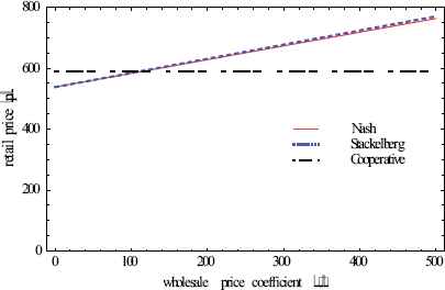
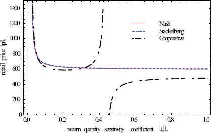
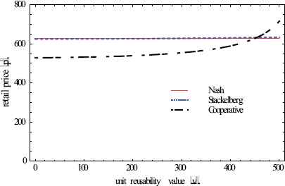
To explore the effect of each coefficient on the retail price, we use the parameters in Table 2 for study, the trends of the retail prices in different games are show in Fig. 2. As show in Fig. 2, it is found the retail prices for simultaneous-move and sequential-move game are almost the same, and the tendencies are similar to the cooperative game.


The effects on retail price
Fig. 2(a) shows the influence of demand on retail price sensitivity coefficient, the retail price decreases dramatically with β increasing, and be stable when β reaches to 0.6, we also find the MC supply chain can be more endurable to lowing price in the case of cooperative game. Fig. 2(b) allows us to see the influence of refund-demand sensitivity coefficient, retail price γ increases up to 0.6 and then approaches the positive infinity. The result shown in Fig. 2(c) reveals the variable coefficient ε has almost no influence on simultaneous-move game’s and sequential-move game’s retail price, while for the cooperative game, the retail price decreases slowly while ε increases. From Fig. 2(d), the wholesale price coefficient θ has no effect on cooperative game’s retail price, but for the simultaneous-move game and sequential-move game, there is a positive moderate linear relationship between retail price and θ. As show in Fig. 2(e), the influences of return quantity coefficient ψ are significant for the non-cooperative and cooperative games in the range of ψ ≤ 0.1, while in the range of ψ > 0.1, the retail price almost remains stable, the jump discontinuity point in cooperative game is the zero point existing in the denominator, that has little practical effect. In fig. 2(f), unit reusability value v has no effect on non-cooperative games’ retail price and has no significant effect on the cooperative game. The results indicate that, when the customized market is sensitive to retail price, the supply chain has to lower retail price to consolidate the market share, meanwhile, the MC supply chain can simulate the market demand by higher γ value.
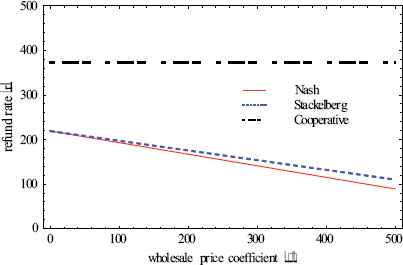
5.2.2 Effects on refund rate
Fig. 3 shows the influence on the refund rate r. From Fig. 3(a) to Fig. 3(f), the refund rate in cooperative game is generally more than the two non-cooperative games. Fig. 3(a) reveals that there is an inverse correlation between the refund rate and price sensitivity coefficient β, the refund rate decreases significantly while increases in the range of β ≤ 0.4. From Fig. 3(b), the influences of γ is notable both for the Non-cooperative and Cooperative games, refund rate γ increases up to 0.6 and then approaches the positive infinity. As show in Fig. 3(c), the variable cost coefficient ε has little influence on non-cooperative games’ refund rate, while for the cooperative game, r plummets with ε increasing. In Fig. 3(d), the wholesale price coefficient θ has no effect on cooperative game’s refund rate, also, has little influence on non-cooperative games’. As show in Fig. 3(e), the refund rates of all of three games plummet in the range of ψ ≤ 0.2. However, in the range of ψ > 0.2, the slope for non-cooperative games’ refund rate are relatively flat, while for the cooperative game, the refund rate begins to rebound significantly. Fig. 3(f) reveals that the unit reusability value v has little effect on non-cooperative games’ refund rate, but for the cooperative game, the refund rate increases with v increasing.


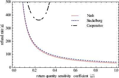

The effects on refund rate
Hence, the customized products in cooperative game should be more attractive when the customer demand is more sensitive to the return policy. Though the refund rate is higher than the Non-cooperative supply chain, it is more profitable for the cooperative supply chain due to the larger market demand (refer to Fig. 5).

The effects on market demand
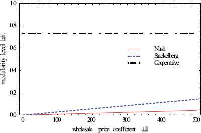
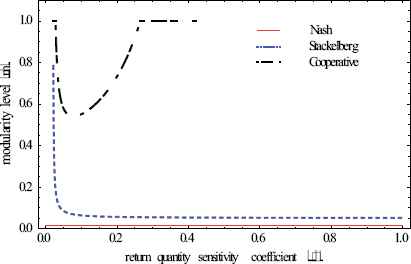
5.2.3 Effects on modularity level
Fig. 4 shows the influence on the modularity level. We can see that the modularity level in simultaneous-move game is very small and almost steady, while in the sequential-move game, the modularity level has been increases significantly, the highest modularity level occurs in the cooperative game. Fig. 4(a) shows that the modularity level has inverse relationship with the price sensitivity coefficient β. The most obvious impact on modularity level occurs in the sequential-move game in range of β ≤ 0.1, when β > 0.1, the modularity level remains below 0.2, while in the cooperative game, the modularity level remains at 1 and does not decrease until β = 0.4. From Fig. 4(b), we can see that modularity levels are proportional to the refund-demand sensitivity coefficientγ, it reaches to 1 at the point of γ = 0.6 in sequential-move game, however, in cooperative game, it dramatically increases from 0.2 to 1. In Fig. 4(c), the modularity level decreases while ε increases, furthermore, the modular production dose not exist in the MC supply chain when ε ≥ 100. Fig. 4(d) reveals that the wholesale price coefficient θ only impacts the profit sharing in the MC supply chain, not the modularity level. As show in Fig. 4(e), the modularity levels in sequential-move game and cooperative game decrease rapidly in the range of ψ ≤ 0.1. However, in the range of ψ > 0.1, the sequential-move game’s refund rate is almost stable (m= 0.1), while the Cooperative game’s refund rate decreases to 0.5 at ψ = 0.1, then rebounds to m =1 at ψ = 0.3. Fig. 4(f) reveals that, the unit reusability value v has little effect on non-cooperative games’ modularity levels. But for the cooperative game, there is a positive linear relationship between m and v, the modularity level greatly increases up to 1 in the range of v ≥ 200.


The effects on modularity level
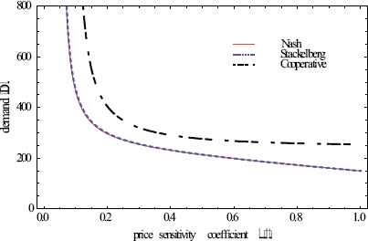
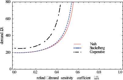
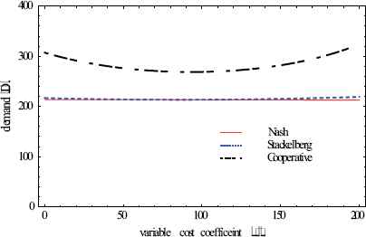
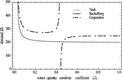
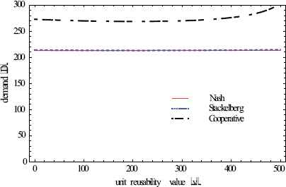
5.2.4 Effects on market demand
Fig. 5 reflects the effects of each individual coefficients on the market demand. From Fig. 5(a) to Fig. 5(f), we can see that, the market demands are almost the same in the two non-cooperative games but far less than in the cooperative game. As show in Fig. 5(a), under the influence of price sensitivity coefficient, the market demand drops significantly in range of β ≤ 0.2. Fig. 5(b) reveals that the market demand will approaches the positive infinity when γ = 0.6. In Fig. 5(c), the variable cost coefficient ε has no influence on non-cooperative games’ market demand, but for the cooperative game, when ε increases, the market demand decreases and then increases, but the fluctuation range is small. From Fig. 5(d), the market demand has inverse relationship with the basic return quantity ϕ. As Fig. 5(e) illustrates, when the influence of the return quantity sensitivity coefficient ψ on customer’s choice increases, the market demand decreases, this is mainly due to the fact that the refund rate provided by the module manufacturer is low, in addition, the jump discontinuity point in Fig. 5(e) is the zero point existing in the denominator, it has little practical effect. Fig. 5(f) reveals the unit reusability value v has little effect on market demand.
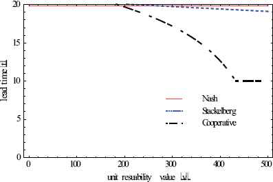
5.2.5 Effects on lead time
Fig. 6 describes the influence on lead time. We can see from Fig. 6 that the lead time in simultaneous-move game is very long and almost steady in any case, while in the sequential-move game, the lead time has a tendency to be relatively short. However, for the cooperative game, the lead time is the shortest and remains unstable, it means through cooperation supply chain could greatly minimize lead time, but hardly control it to some extent.
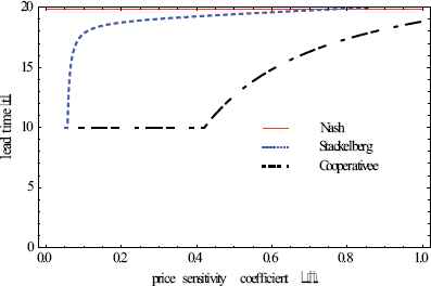
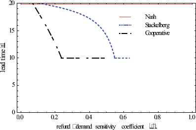
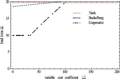
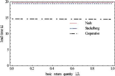
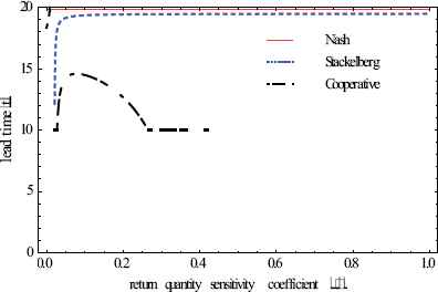
The effects on lead time
Fig. 6(a) shows that the lead time has positive relationship with the price sensitivity coefficient β. The up trend of sequential-move game’s lead time is obvious in range of β ≤ 0.1, then remains stable. While in the cooperative game, the lead time remains at 10 and dose not increase until β =0.4. Fig. 6(b) shows a negative relation between lead time and the refund-demand sensitivity coefficient γ. However, in cooperative game, it reaches to the minimum value (10) at the point of γ = 0.2 with the most significant trend, it also achieves stability at the point of γ = 0.6 in sequential-move game. In Fig. 6(c), the lead time increases with ε increasing, and reaching the maximum points at ε = 100. Fig. 6(d) reveals that the basic return quantity ϕ has no effect on lead time. As show in Fig. 6(e), the lead times in sequential-move game and cooperative game increase rapidly when ψ is not larger than 0.1. However, in the range of ψ > 0.1, the sequential-move game’s lead time almost keeps stable, while for cooperative game’s lead time, it starts to decrease at the point of ψ = 0.1 form the maximum value (15) to the minimum value (10). Fig. 6(f) reveals that the unit reusability value v has little effect on non-cooperative games’ lead times, but for the cooperative game, there is a positive linear relationship between t and v, the lead time decreases markedly in the range of v ≥ 200 until t =10.
6. Conclusion and future research
In this paper, we have investigated the competition and cooperation between the upstream module manufacturer and the downstream customized assembler under the MC supply chain scenario. Through employing the game theory, we have identified the optimal pricing, modularity level, return policy and lead time in three types of decision-makings. In addition, coordination mechanism is design to cooperate in MC supply chain via profit-sharing scheme. Finally, we have used numerical analysis and gained some insights into how different parameters affect the optimal decisions.
We have found that retail price, refund rate and market demand in competition environment (simultaneous-move and sequential-move games) are almost the same. However, the refund rate for MC supply chain under cooperation setting (cooperative game) is larger than that under non-cooperative setting, it is more profitable for the whole supply chain due to the larger market demand. The modularity level in simultaneous-move game is very low and almost steady, while in the sequential-move game, the modularity level has been increased significantly, however, the highest modularity level occurs in the cooperative environment. The lead time in simultaneous-move game is very long and almost steady, while in the sequential-move game, the lead time has a tendency to be short but relatively flat. However, the cooperative MC supply chain can greatly reduce lead time, which is important for MC supply chain to quickly respond to market change and remain competitive advantage.
We also examined the uncertainty issue associated with MC implementation under supply chain through sensitive analysis. It appears that different optimal decisions will result depending on the factor change. we have found that the variable cost and unit reusability value have little effect on the optimal decision in competition settings, while in the cooperative one, the influence of wholesale price is not significant. At the same time, we have revealed the price sensitivity coefficient β and the refund-demand sensitivity coefficient γ are influential both for the competition and cooperative settings, thus, the MC supply chain should pay more attention to the pricing strategy and refund policy. What’s more, we also have found that the MC supply chain only employ cooperative strategy, which is helpful in achieving Pareto improvement for the members along MC supply chain.
This work reveals some promising areas where one could place more efforts in the future. More sophisticated aspects in MC supply chain be added into the model. For example, risk issue of the upstream and downstream firms may vary in different decision-makings. The risk attitude of MC supply chain member has influence on results, thus risk preference could be applied into this framework.
Acknowledgement
This research was supported by the National Science Foundation China (Grant No. 71472143, 71171152) and Education Department program in Hubei Province (Grant No. 15ZD026).
References
Cite this article
TY  - JOUR
AU  - Jizi Li
AU  - Chunling Liu
AU  - Weichun Xiao
PY  - 2016
DA  - 2016/12/01
TI  - Modularity, Lead time and Return Policy for Supply Chain in Mass Customization System
JO  - International Journal of Computational Intelligence Systems
SP  - 1133
EP  - 1153
VL  - 9
IS  - 6
SN  - 1875-6883
UR  - https://doi.org/10.1080/18756891.2016.1256575
DO  - 10.1080/18756891.2016.1256575
ID  - Li2016
ER  -