
A metaheuristic optimization-based indirect elicitation of preference parameters for solving many-objective problems
- DOI
- 10.2991/ijcis.2017.10.1.5How to use a DOI?
- Keywords
- metaheuristic; decision aid; parameter inference; indirect approach; preference analysis disaggregation
- Abstract
A priori incorporation of the decision maker’s preferences is a crucial issue in many-objective evolutionary optimization. Some approaches characterize the best compromise solution of this problem through fuzzy outranking relations; however, they require the elicitation of a large number of parameters (weights and different thresholds). This paper proposes a novel metaheuristic-based optimization method to infer the model’s parameters of a fuzzy relational system of preferences, based on a small number of judgments given by the decision maker. The results show a satisfactory rate of error when predicting new outcomes with the parameter values obtained by using small size reference sets.
- Copyright
- © 2017, the Authors. Published by Atlantis Press.
- Open Access
- This is an open access article under the CC BY-NC license (http://creativecommons.org/licences/by-nc/4.0/).
1. Introduction
A wide variety of problems in the real world often involve multiple objectives to be minimized or maximized simultaneously1,2. As a consequence of the conflicting nature of the criteria, it is not possible to obtain a single optimum, and consequently, the ideal solution to a multi-objective optimization problem (MOP) cannot be reached. Unlike single-objective optimization, the best solution of a MOP is not well-defined from a purely mathematical point of view. To solve a MOP means to find the best compromise solution according to the decision maker’s (DM’s) particular system of preferences. Since all the compromise solutions are mathematically equivalent, the DM should provide some additional information for choosing the most preferred one3.
Multi-Objective Evolutionary Algorithms (MOEAs) are particularly attractive to solve MOPs because they deal simultaneously with a set of possible solutions (the MOEA’s population), which allows to obtain an approximation of the Pareto frontier in a single run of the algorithm. Thus, by using MOEAs the DM and/or the decision analyst does not need to perform a set of separate single-objective optimizations (as is usually required when using conventional multi-objective programming methods) in order to generate compromise solutions. Additionally, MOEAs are more robust regarding the mathematical characteristics of objective functions and constraints, whereas these are real concerns for mathematical programming methods (cf. Ref. 4).
Most current approaches in evolutionary multi-objective optimization concentrate on generating an approximation of the Pareto optimal set. The DM still has to choose the best compromise solution out of that set. Nevertheless, as was stated in Ref. 5, there has been an increasing interest in incorporating the DM’s preference information in the search process. Following Ref. 5, this interest is motivated by the following issues:
- 1.
The DM’s cognitive effort would be greatly reduced if the MOEA were able to identify the Region of Interest (RoI), the privileged zone of the Pareto frontier that best matches the DM’s preferences. This is particularly important in problems with five or more objectives because i) the capacity of the human mind is restricted to handling a small amount of information at the same time6; and ii) the cardinal of a representative portion of the known Pareto frontier grows exponentially with the number of objective functions.
- 2.
With an increasing number of objectives, almost all solutions in a current MOEA’s population become non-dominated (in a local sense); so, the algorithm’s selective pressure toward the true Pareto frontier may be very weak; the DM´s preference information allows reinforcing the necessary selective pressure.
Most approaches for incorporating preferences in MOEAs assume a particular model of DM preferences. This model may be based on value functions (cf. Refs. 7, 8, 9), outranking relations (see Ref. 3), reference points (cf. Ref. 10), reservation points11, desirability thresholds12, decision rules13, and other ways of aggregating multi-criteria preferences. Interesting surveys of this topic are found in Refs. 14 and 15.
The models based on outranking relations exhibit some desirable features: i) the outranking approach can handle imprecise and qualitative information; ii) the preference relation derived from the outranking information can be used as complement of dominance, increasing the selective pressure toward the RoI; iii) fuzzy outranking relations are more flexible than value functions, handling phenomena as intransitivity and incomparability.
An interesting outranking approach for incorporating preferences in MOEAs was proposed by Fernandez et al. in Ref. 3. Based on the index of credibility of the outranking, Fernandez et al. modeled the relational system of preferences proposed by Roy in Ref. 16. They derived a model for the strict, weak and K-preference. An original many-objective problem is mapped in a surrogate three-objective problem, as proposed in Ref. 3. The best compromise solution is a non-dominated solution of the surrogate problem.
The method of Fernandez et al. in Ref. 3 was successfully applied in solving portfolio problems with many objectives17,18 and project partial support19. In order to apply the method, the outranking model parameters (weights and thresholds required by the index of credibility of the outranking) must be elicited. Besides, some additional symmetric and asymmetric parameters (that are specific of the preference model proposed by Fernandez et al. in Ref. 3 are required too. Usually, the DMs reveal difficulties when they are inquired to assign values to parameters whose meanings are barely clear for them20. On the other hand, indirect procedures, which compose the so-called preference-disaggregation analysis (PDA), use regression-like methods for inferring a set of parameters from a battery of decision examples21. According to Greco et al. in Ref. 22, MCDA approaches based on disaggregation paradigms are of increasing interest because they imply relatively less cognitive effort from the DM. The direct eliciting settlement has been criticized in Refs. 23 and 24. Marchant argues23 that the only valid preferential input-information is that arising from DM’s preferential judgments in pairwise comparisons.
The heavy cognitive effort required from the DM in order to make a direct parameter setting is probably the main objection against the approach of Ref. 3. As a consequence, a method for an indirect parameter elicitation would be welcome to concern many objective problems. However, as stated by Fernandez20, in outranking-based models, inferring all the parameters simultaneously requires solving a non-linear programming problem with non-convex constraints, which is usually difficult for mathematical programming techniques25,26. According to Doumpos21, the relational form of these models and the veto conditions may make it impossible to infer the model parameters in real-size data sets by using mathematical programming. An alternative is the use of metaheuristics, which can find, in relatively small time, approximated solutions convenient for real purposes (see, e.g. Refs. 27 and 28).
The research work in this paper focuses on the development of an optimization approach for the PDA method. The approach is based on metaheuristics and used to infer the parameters of the preference model proposed by Fernandez3. According to the consulted scientific literature, our work is the only one so far that involves the considered outranking parameters. The resulting method was tested using different algorithms. The conducted experimental design evaluated the quality of the estimated parameters in both, its proximity to the real parameters, and its capacity to predict new preference relations. The remaining of this document is organized as follows. Section 2 defines the preference relations, and the surrogate model defined in Ref. 3. Section 3 shows the particular set of parameters studied, and the inference approach defined in this paper to estimate them. Section 4 shows the developed method to estimate parameters for the studied preference model, and presents the experimental design conducted in order to test the method. Finally, Section 5 presents some concluding remarks derived from our research.
2. The method of Fernandez et al. (2011) for finding the best compromise
Consider a MOP of the form
In the following O denotes the image of RF in the objective space mapped by the vector function F. An element x ∈ O is a vector (x1, …, xn), where xi is the i-th objective function value. S(x,y) denotes the predicate “the DM considers that option x is at least as good as y” defined on O×O.
Roy described16 situations concerning this non-ideal behavior from real decision actors by using a relational system of preferences composed of several binary relations. The definitions from Roy16 are given below:
- 1.
Indifference: It corresponds to the existence of clear and positive reasons that justifies equivalence between the two actions. Notation: xIy.
- 2.
Strict preference: It corresponds to the existence of clear and positive reasons that justify significant preference in favor of one (identified) of the two actions. The statement x is strictly preferred to y is denoted by xPy. P is asymmetric and non-reflexive.
- 3.
Weak preference: It corresponds to the existence of clear and positive reasons in favor of x over y, but that are not sufficient to justify strict preference. Indifference and strict preference cannot be distinguished appropriately. This is denoted by xQy. Q is asymmetric and non-reflexive.
- 4.
Incomparability: None of the preceding situations predominates. That is, the absence of clear and positive reasons that justify any of the above relations. Notation: xRy. R is symmetric.
- 5.
K-preference: It corresponds to the existence of clear and positive reasons that justify strict preference in favor of one (identified) of the two objects or incomparability between the two objects, but with no significant division established between the situations of strict preference and incomparability. Notation: xKy. K is asymmetric.
- 6.
Non-preference: It corresponds to situations in which indifference and incomparability are both possible, without being able to differentiate between them. This is denoted by x~y. ~ is symmetric.
Fernandez et al. assumed3 that there is a method for assigning a degree of truth σ(x,y) in [0, 1] to the predicate S(x,y); outranking methods such as ELECTRE-III29,30 and PROMETHEE31 may be used. This work uses ELECTRE-III, as defined in Appendix A. Once σ(x,y) has been calculated, it can be useful for modeling the crisp preference relations defined b for each pair (x, y):
Definition 1:
x is (λ,β)-strictly preferred to y if at least one of the following conditions holds y Roy (1996). Using real numbers λ, β, ε, (ε<β<λ<1), the proposals in Refs. 3 and 17 define the following relations:
- i.
x dominates y
- ii.
σ(x,y) ≥ λ ∧ σ(y,x) < 0.5
- iii.
σ(x,y) ≥ λ ∧ (0.5 ≤ σ (y,x) < λ) ∧ (σ(x,y) - σ(y,x))≥β
Notation: xP(λ,β)y. The value λ is the outranking credibility threshold, greater than 0.5; β is an asymmetry parameter.
Definition 2:
x and y are (λ,ε)-indifferent if σ(x,y) ≥ λ, σ(y,x) ≥ λ and |σ(x,y) - σ(y,x)| < ε. Notation: xI(λ,ε)y. The value ε is a symmetry parameter.
Definition 3:
x is (λ,β,ε)-weakly preferred to y if the following conditions are satisfied.
- i.
σ(x,y) ≥ λ ∧ σ(x,y) > σ(y,x)
- ii.
x . not P(λ,β)y
- iii.
x . not I(λ,ε)y
Notation: xQ(λ,β,ε)y
Definition 4:
x is (λ,ε)-K-preferred to y if the following conditions are satisfied:
- i.
0.5 ≤ σ (x,y) < λ
- ii.
σ (y,x) < 0.5
- iii.
(σ(x,y) - σ(y,x)) > ε
Notation: xK(λ,ε)y
Definition 5:
The incomparability relation xRy is defined by σ(x,y) <0.5 ∧ σ(y,x) <0.5.
Definition 6:
There is a (λ,β,ε)-non-preference between x and y if the following conditions are satisfied.
- i.
not. xP(λ,β)y ∧ not. yP(λ,β)x;
- ii.
not. xQ(λ,β,ε)y ∧ not. yQ(λ,β,ε)x;
- iii.
not. xK(λ,ε)y ∧ not. yK(λ,ε)x;
- iv.
not. xI(λ,ε)y;
- v.
not. xRy.
Notation: x~(λ,β,ε)y
Fernandez et al. used3 the above relations P, Q and K to define the best compromise solution to Problem 1 as follows:
- •
Given x ∈O, the set of (λ,β,ε)-strictly outranking solutions is defined as (SO)x = {y ∈O such that yP(λ,β)x};
- •
The (λ,β,ε)-non strictly outranked frontier is defined as NS = {x ∈O such that card (SO)x = 0};
- •
If x* is the best compromise of Problem 1, then there is no y∈O such that yPx*. Then, if P⊆P(λ,β), in order to be the best compromise x* must belong to NS (a necessary condition).
Once NS has been identified, Fernandez et al. suggest3 to choose the best compromise considering two additional criteria: a) card (WNS)x= card {y ∈NS such that yQ(λ,β,ε)x or yK(λ,β)x}; and, b) card (FNS) = card {y ∈NS such that Fn(y) > Fn(x)}, where Fn denotes the net flow score in NS, that is Fn(a) = Σ c∈ NS -{a} [σ(a,c) - σ(c,a)]. The best solution to Problem 1 is chosen from the non-dominated set of
3. A method to infer the model parameters by using preference relations
This section presents the inference approach used to estimate the parameter values of the fuzzy relational system.
3.1. Some assumptions
Assumption 1:
The DM is willing to make judgments using P, Q, I, K, R and ~ on a reference set T of pairs of alternatives (x, y).
Assumption 2:
Given a pair of alternatives (x, y) the DM can identify one and only one of the following statements as more acceptable: xPy, yPx, xIy, xQy, yQx, xKy, yKx, xRy, x~y. So, each pair (x,y) in T is associated with a relation A of the set {P, I, Q, K, R, ~, P−1, Q−1, K−1}, where (xA−1y ⇔ yAx).
3.2. The model parameters
If credibility index σ(x,y) is calculated as in ELECTRE III, the following parameters must be specified in the model of Fernandez et al. in Ref. 3:
- i)
the vector of weights w={w1, w2, …, wn};
- ii)
the vector of indifference thresholds q={q1, q2, …, qn};
- iii)
the vector of preference thresholds p={p1, p2, …, pn};
- iv)
the vector of veto thresholds u={u1, u2, …, un};
- v)
the vector of discordance thresholds (only when the simplification suggested by Mousseau and Dias is used32) v={v1, v2, …, vn};
- vi)
λ, β, and ε.
Given the alternatives (x,y), the value of the credibility index σ(x,y) is a function of the parameters η={w,q,p,u,v}, and will be denoted in the future as σ(η,x,y). The function σ(η,x,y), in combination with the remaining outranking (λ), symmetry (β), and asymmetry (ε) thresholds, determine the preference relations according to Definitions 1–6.
3.3. The inference approach
Let Pfr be the set of feasible parameter vectors (η,λ,β,ε). The ideal solution of the parameter elicitation problem would be (η0,λ0,β0,ε0) ∈Pfr such that the following equivalences are satisfied for all (x, y)∈T :
The best parameter setting should be the closest solution to the ideal one in the sense of certain acceptable metric. Following Refs. 3 and 20 we propose a metric based on the so-called inconsistencies with Eqs. 3. Shortly, an inconsistency arises when an equivalence in Eqs. 3 is not fulfilled. For example, given (x, y)∈T and (η,λ,β,ε)∈Pfr we call inconsistency with (3.a) the fact that x is strictly preferred to y by the DM and however not (xP(η,λ,β)y), or vice versa, xP(η,λ,β)y but x is not strictly preferred to y by the DM. Let N1, N2, …, N6 be the number of inconsistencies in T with Eqs. 3.a, 3.b, 3.c, 3.d, 3.e and 3.f, respectively.
Since the method by Fernandez et al. in Ref. 3 (see Problem 2) gives priority to find the non-strictly outranked set, N1 is far the most important measure. The information coming from Q and K is also considered in Problem 2, being thus more important than that provided by I, R, and ~. So, we propose to find the best (η,λ,β,ε) from the solution of the optimization problem:
4. Optimization approach to solve the inference approach
This section presents the proposed approach based in metaheuristic to estimate the parameter values of the model of preferences studied.
4.1. Some metaheuristic approaches
We propose here a method based on mono-objective optimization algorithms to solve Problem (4). The method exploits the preemptive priority established for the problem; it finds the best value for the first objective, then this value is used as a bound when the second objective is minimized. Finally, E3 is minimized keeping the minimum values previously obtained for (E1, E2).
Figure 1 depicts the general procedure followed by the approach. Each metaheuristic algorithm solves P=(DMsim,T), i.e. an instance of Problem (4) formed by the parameter values that define the model of preferences for a simulated DM, denoted as DMsim, and its reference set T, trying to minimize only the objective E1. The best value BestE1 is used as bound in the following step of the method; in this step the same algorithm searches the minimization of objective E2 while it validates that the solutions achieved yield a value on E1 equal or smaller than BestE1. Finally, in the last step, the algorithm now minimizes the third objective of Problem (4), i.e. E3, while keeping the values for E1 and E2 smaller than BestE1 and BestE2, respectively. The best solution (η*,λ*,β*,ε*) will arise from the parameter vectors obtained from the last step of this procedure.
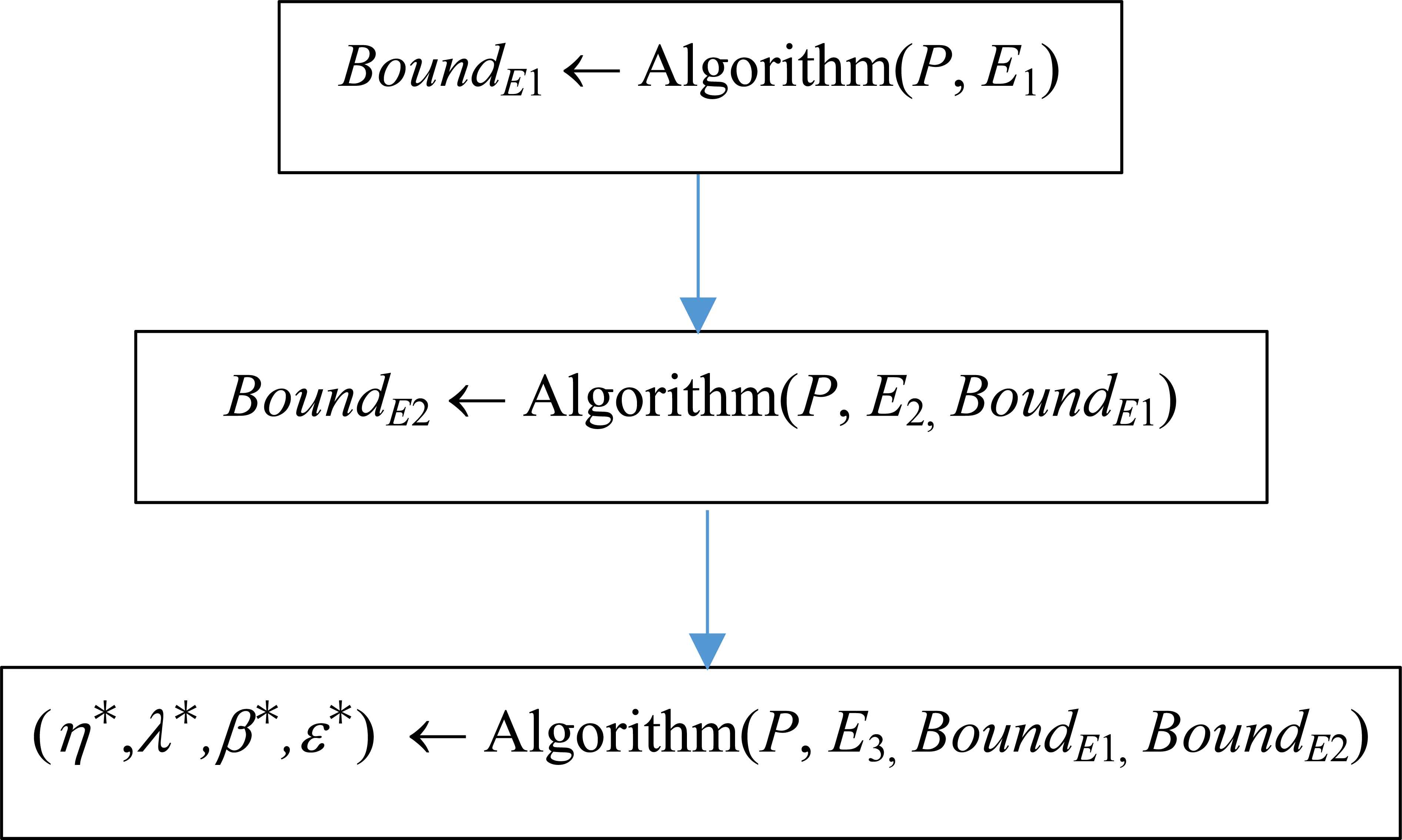
Strategy followed to solve Problem (4) using mono-objective algorithms.
The algorithms that were analyzed in this work are: a) Genetic Algorithm; b) Particle Swarm Optimization; c) Tabu Search; and, d) Simulated Annealing. These strategies have two main components in common: the problem encoding and the evaluation function. The evaluation function on each stage of the general procedure is related to a particular objective Ei of Problem (4), and is described in Section 3.3. The encoding, the algorithms, and the fine-tuning process of the algorithms’ parameters are detailed in the remaining of this section.
4.1.1. Problem encoding
All the strategies developed in this work use the same encoding to solve Problem (4). This encoding is based on a vector ρ of real numbers which represents the parameter vector (η,λ,β,ε) to be estimated. The size of ρ is 5n+3, depending on the number n of criteria involved.
In order to provide an example of the proposed encoding, let’s suppose that the decision process is made over actions composed by two criteria. Then, the vector ρ will be set up as in Figure 2.
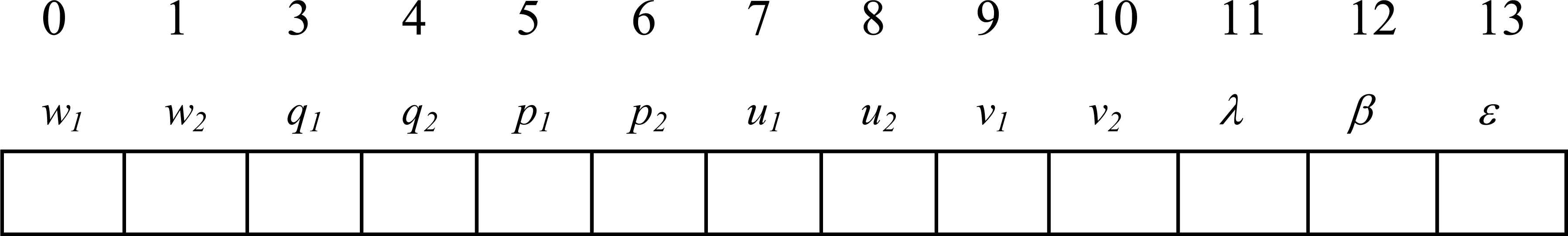
Vector ρ representing a solution for the Problem (4).
4.1.2. Genetic Algorithm
The Genetic Algorithm metaheuristic (GA) is inspired by natural selection, it uses data structures that represent chromosomes, and it moves from one population of them to another new one through recombination, mutation, crossover, or selection operators, in order to preserve critical information (see Refs. 33 and 34).
The algorithm shown in Figure 3 is based on a GA paradigm, and it is used to solve Problem (4) under the lexicographic method previously described.
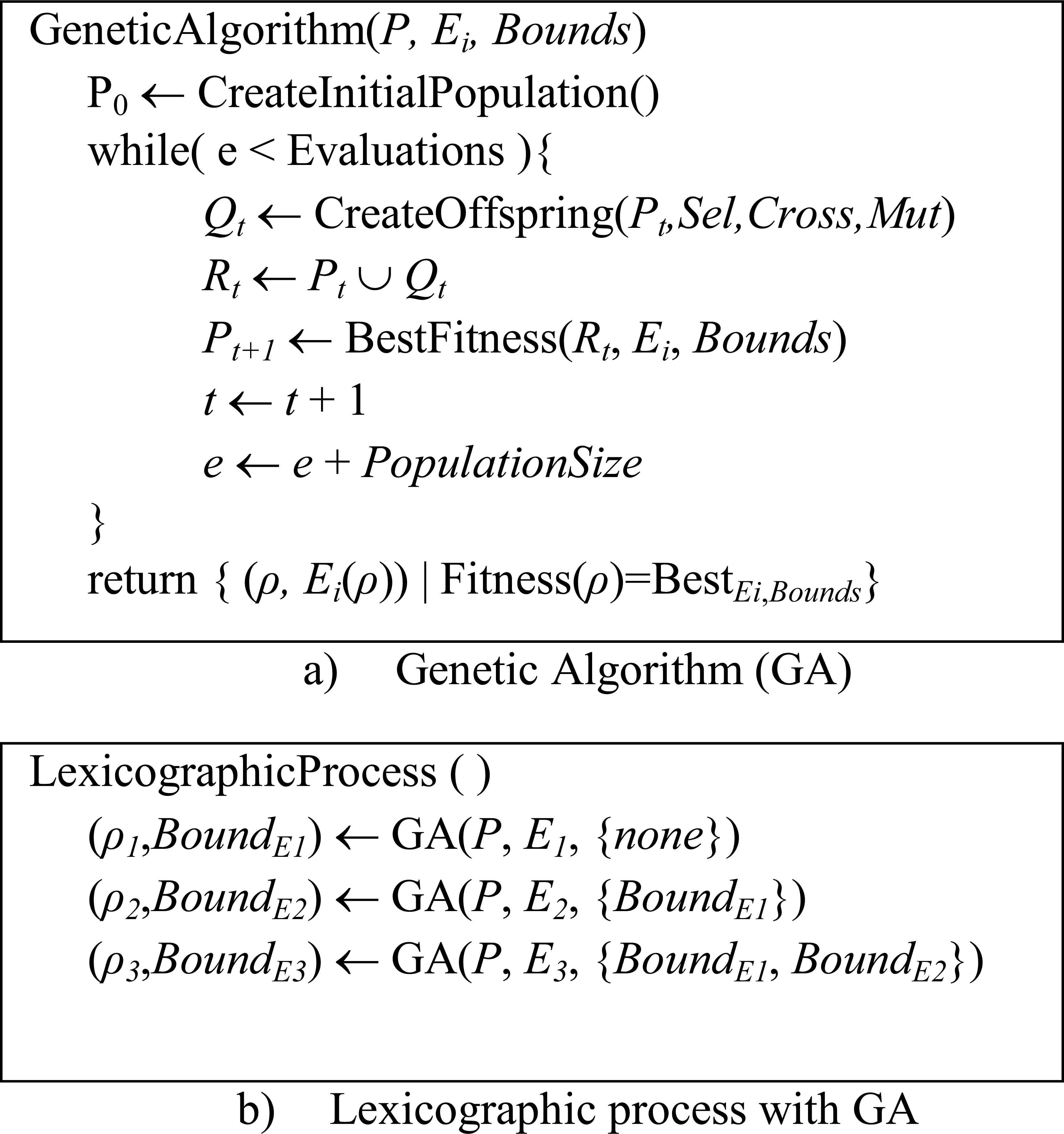
Method for Problem (4) based on GA.
The chromosome of the GA is derived from the encoding in Section 4.1.1. The algorithm randomly creates an initial population of individuals P0. After that, and at each generation, it creates from the actual Pt a new offspring population Qt using the chosen operators. Basically, in this phase the algorithm uses Binary Tournament to choose two parents, and breed two child using Simulated Binary Crossover (or SBXCrossover); finally, the pair of resulting offprings is subject to the Polynomial Mutation process.
The next step in the algorithm is the combination of parents and offspring into a set Rt from which will be extracted the individuals with the best fitness; these will form the next generation of parents Pt+1, and their fitness is evaluated from the objectives Ei in Problem (4) taking into account the constraints. The number of individuals per generation is defined in the parameter Population Size.
Note that this implementation of the GA defines the stop criterion in terms of the maximum number of evaluations allowed; on this base the number of generations can be computed through the quotient of the Evaluations and the Population Size.
The GA will return the set of parameter vectors that yield the best fitness value for the objectives Ei satisfying the Bounds.
The key elements required in the implementation of the proposed GA are: a) for the polynomial mutation, its probability and index of distribution; b) for SBXCrossover also its probability and index of distribution; c) the population size; and d) the stop criterion (or Evaluations).
The parameters of the GA were subject of a fine-tuning process based on Covering Arrays (CA) (see Ref. 35), in order to identify the best configuration of them for the GA.
The fine-tuning process employs commonly used parameter values (in this case are the ones in Table 1a), and with the CA it constructs a set of valid configurations (see Table 1b); finally, using a random generated instance, it tests all the configurations to identify the one with the best performance, which in our case is shown in Table 1c. The best one is used to lead the main experimental design proposed in this paper.
| Possible Values | ||||
|---|---|---|---|---|
| No. | Parameter | V1 | V2 | V3 |
| A | Mut. | 0.02 | 0.05 | 0.10 |
| B | Mut. | 5 | 10 | 20 |
| C | Cross. | 0.85 | 0.90 | 0.95 |
| D | Cross. | 5 | 10 | 20 |
| E | Population | 50 | 100 | 200 |
| F | Evaluations | 100000 | 50000 | 25000 |
a) Tested Parameter Values
| Parameter Values | ||||||
|---|---|---|---|---|---|---|
| Config. | A | B | C | D | E | F |
| 1 | 0.02 | 5 | 0.90 | 20 | 200 | 50000 |
| 2 | 0.02 | 10 | 0.90 | 5 | 100 | 100000 |
| 3 | 0.02 | 20 | 0.85 | 5 | 50 | 25000 |
| 4 | 0.05 | 5 | 0.95 | 5 | 50 | 100000 |
| 5 | 0.05 | 10 | 0.85 | 10 | 200 | 100000 |
| 6 | 0.05 | 20 | 0.90 | 20 | 100 | 25000 |
| 7 | 0.10 | 5 | 0.85 | 10 | 100 | 25000 |
| 8 | 0.10 | 10 | 0.95 | 20 | 50 | 50000 |
| 9 | 0.10 | 20 | 0.90 | 10 | 50 | 100000 |
| 10 | 0.02 | 20 | 0.95 | 10 | 200 | 50000 |
| 11 | 0.10 | 10 | 0.95 | 5 | 200 | 25000 |
| 12 | 0.05 | 10 | 0.85 | 20 | 100 | 50000 |
| 13 | 0.05 | 20 | 0.95 | 5 | 100 | 25000 |
| 14 | 0.02 | 20 | 0.90 | 20 | 100 | 100000 |
| 15 | 0.05 | 10 | 0.95 | 5 | 50 | 50000 |
b) Valid configurations using a CA(15;2,6,3)35
| No. | Parameter | Value |
|---|---|---|
| A | Mut. Probability | 0.02 |
| B | Mut. Distribution Index | 20 |
| C | Cross. Probability | 0.90 |
| D | Cross. Distribution Index | 20 |
| E | Population Size | 100 |
| F | Evaluations | 100000 |
c) Best Configuration, Config. 14
Parameters of GA.
4.1.3. Particle Swarm Optimization
The Particle Swarm Optimization metaheuristic (PSO) is inspired in social models where physical movements, or cognitive experiences are adjusted to optimize environmental parameters of a given population36. The adjustments of the movements are controlled in this algorithm mainly by the parameters ω, φp, and φg, which must be selected carefully to control the behavior and efficacy of the method.
The algorithm shown in Figure 4 is based on a PSO paradigm, and it is used to solve Problem (4) under the lexicographic method previously described37. The definition of particle used by the algorithm is as in Section 4.1.1. The number of dimensions of these particles is set to 5n+3, where n is the number of criteria that define the actions. Firstly, the algorithm defines the initial position xp, the best position bp, and the velocity vp of each particle, and obtain the best known position ρ. Note that the fitness of a position is determined by the objective Ei that is analyzed, and the fulfillment of the constraints (given by Bounds in the pseudocode below). After that, the algorithm updates the velocity vp of the particle and the new value is added to its actual position xp; the velocity vp is updated using the parameters (ω,φp,φg), the values rp, rg generated uniformly at random using U(lp,d, up,d), the best position of the particle bp, and the best known position of the swarm ρ. Finally, the best position bp and the best swarm position ρ are updated accordingly to the new position xp achieved by the particle and its fitness. The algorithm returns ρ.
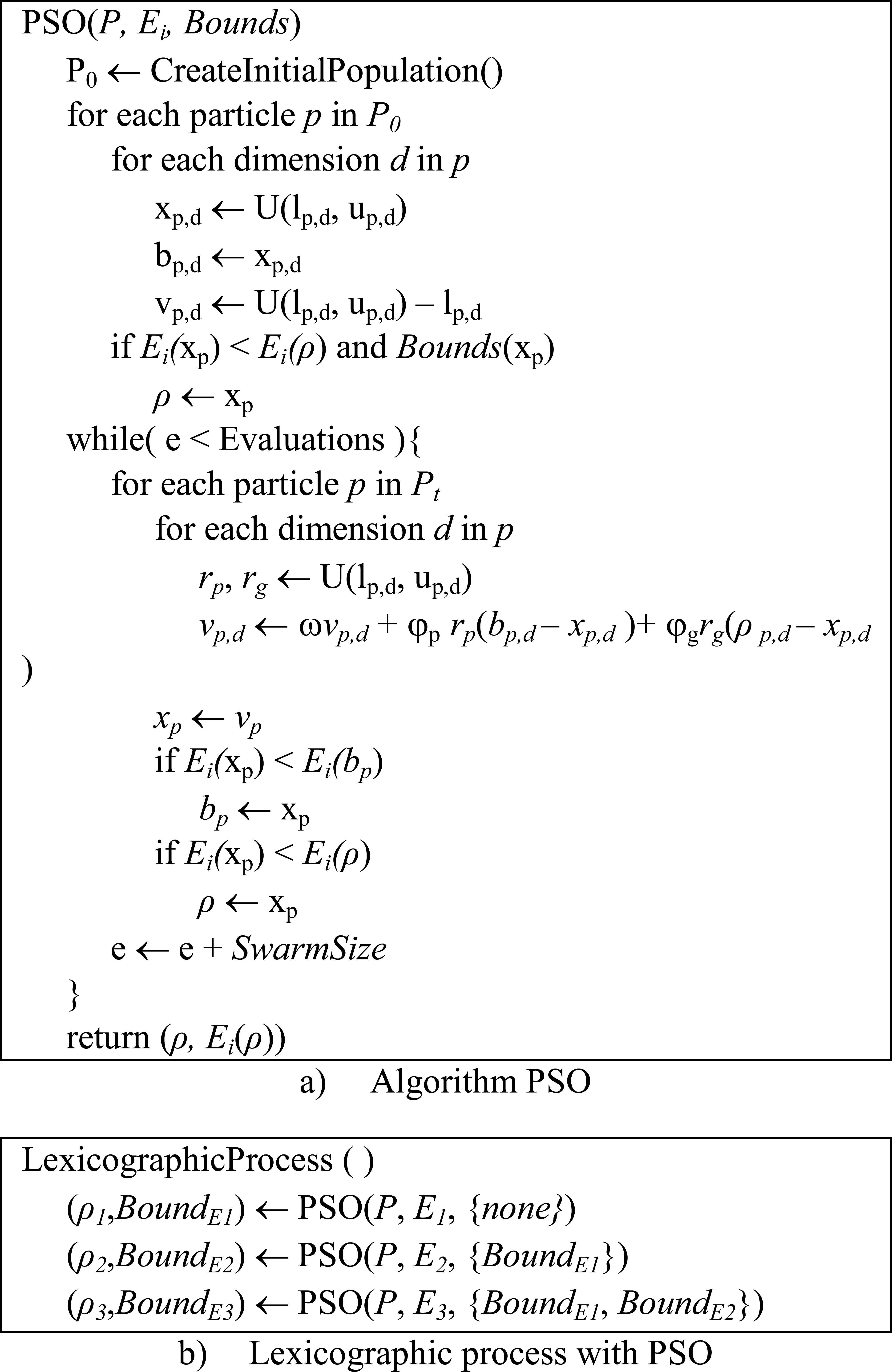
Method for Problem (4) based on PSO.
The parameters of the PSO implementation that require a previous adjustment of their values are ω, φp, φg, the swarm size, and the stop criterion (or Evaluations).
The adjustments in the PSO parameters followed the same CA based method described in Section 4.1.2. Table 2a presents the values considered per parameter; Table 2b shows the set of valid configurations tested; and, Table 2c contains the winner configuration through the method, using a random instance. The latter configuration was used to lead the main experimental design proposed in this paper.
| Possible Values | ||||
|---|---|---|---|---|
| No. | Parameter | V1 | V2 | V3 |
| A | φp | 1.00 | 1.05 | 1.10 |
| B | φg | 1.00 | 1.05 | 1.10 |
| C | ω | 0.10 | 0.20 | 0.30 |
| D | Swarm Size | 50 | 100 | 200 |
| E | Evaluations | 100000 | 50000 | 25000 |
a) Tested Parameter Values
| Parameter Values | |||||
|---|---|---|---|---|---|
| Config. | A | B | C | D | E |
| 1 | 1.00 | 1.00 | 0.20 | 200 | 100000 |
| 2 | 1.00 | 1.05 | 0.20 | 50 | 50000 |
| 3 | 1.00 | 1.10 | 0.10 | 50 | 25000 |
| 4 | 1.05 | 1.00 | 0.30 | 50 | 25000 |
| 5 | 1.05 | 1.05 | 0.10 | 100 | 100000 |
| 6 | 1.05 | 1.10 | 0.20 | 200 | 50000 |
| 7 | 1.10 | 1.00 | 0.10 | 100 | 50000 |
| 8 | 1.10 | 1.05 | 0.30 | 200 | 25000 |
| 9 | 1.10 | 1.10 | 0.20 | 100 | 25000 |
| 10 | 1.00 | 1.10 | 0.30 | 100 | 100000 |
| 11 | 1.10 | 1.00 | 0.30 | 50 | 100000 |
| 12 | 1.05 | 1.00 | 0.10 | 200 | 50000 |
| 13 | 1.10 | 1.00 | 0.30 | 100 | 50000 |
b) Valid configurations using a CA(13;2,5,3)35
| No. | Parameter | Value |
|---|---|---|
| A | φp | 1.05 |
| B | φg | 1.05 |
| C | ω | 0.10 |
| D | Swarm Size | 100 |
| E | Evaluations | 100000 |
c) Best Configuration, Config. 5
Parameters of PSO.
4.1.4. Tabu Search
The Tabu Search metaheuristic (TS) was proposed by Glover and Laguna38. The strategy uses a Tabu list as a memory that stores information of forbidden movements, so that the algorithm can avoid been stuck in a local optimal solution. The strategy uses the expiration time to remove movements from the Tabu list.
The algorithm shown in Figure 5 is based on a TS paradigm, and it is used to solve Problem (4) under the lexicographic method described in Section 4.1.
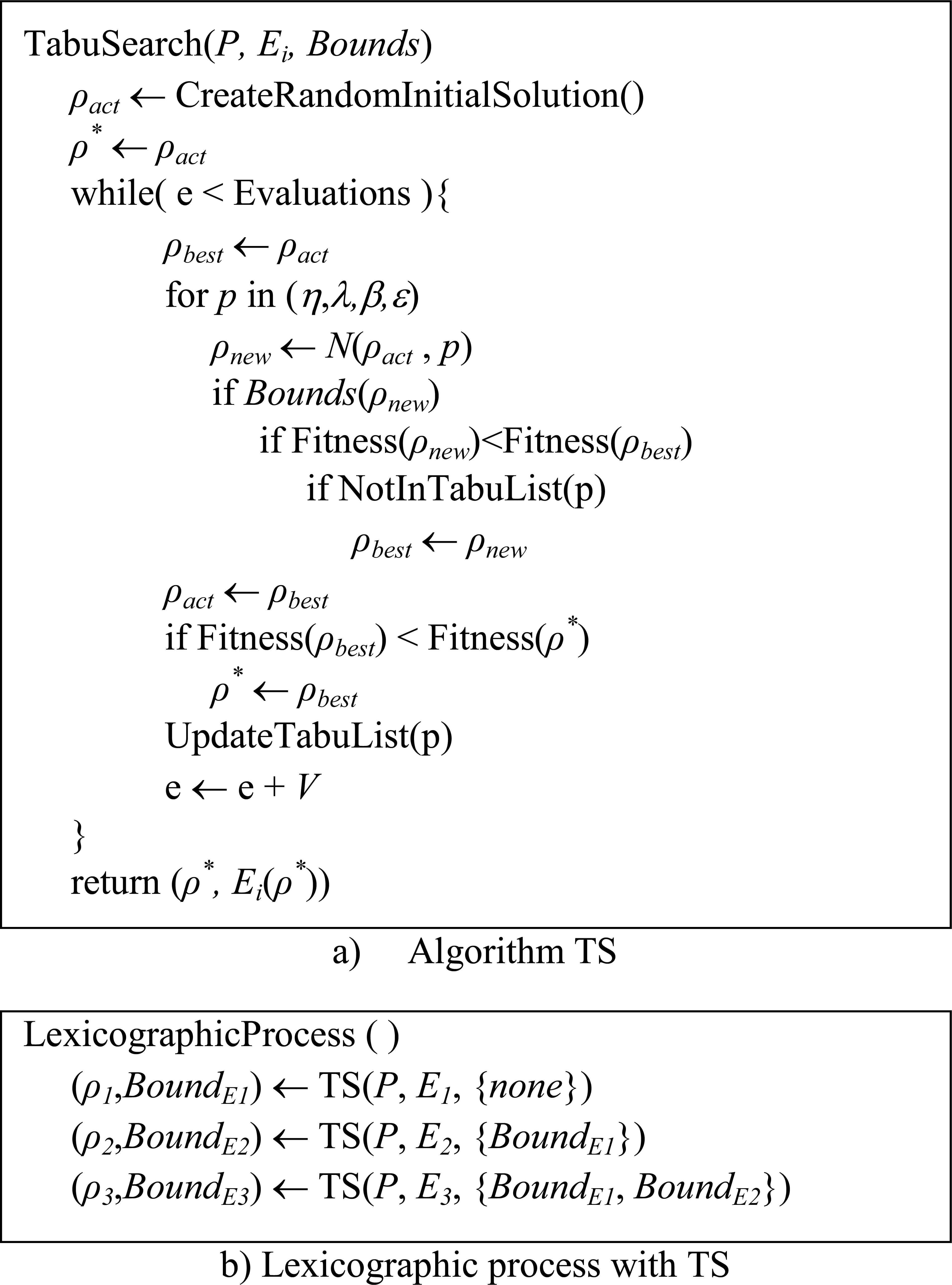
Method for Problem (4) based on TS.
The representation of a solution in the TS of Figure 5 follows the encoding in Section 4.1.1. The neighborhood function used (denoted by N) randomly varies a value of a single chosen parameter in the bounds allowed by the problem; the local search tests every of the V=5n+3 parameters being estimated. The movements in the Tabu list correspond to parameters that are modified to create a new solution from the actual solution ρact. The Fitness of a solution is evaluated using Ei, and the Bounds according to the phase being solved by the method. Firstly, the algorithm tries the change of every parameter of ρact to create a new solution ρnew, and selects the best one ρbest, which has the best fitness and does not belong to the tabu list. After that, the solution ρbest is used to update ρact and the global best solution ρ*. Finally, the tabu list is updated so that the movement p used to produce ρ* is stored, and the expiration time of the remaining is checked. The algorithm returns the global best solution ρ* found.
The CA based fine-tuning process, described in Section 4.1.2, applied to the proposed TS implementation works on the stop criterion (i.e. the number of Evaluations), and on the Tabu list size, and the expiration time used in the UpdateTabuList method. Table 3a presents the values considered per parameter; Table 3b shows the set of valid configurations tested; and, Table 3c contains the winner configuration through the method, using a random instance. The latter configuration was used to lead the main experimental design proposed in this paper.
| Possible Values | ||||
|---|---|---|---|---|
| No. | Parameter | V1 | V2 | V3 |
| A | Expiration | (5n+3) | 2(5n+3) | 5(5n+3) |
| B | Tabu List | (5n+3) | 2(5n+3) | 5(5n+3) |
| C | Evaluations | 25000 | 50000 | 100000 |
a) Tested Parameter Values
| Parameter Values | |||
|---|---|---|---|
| Config. | A | B | C |
| 1 | (5n+3) | 2(5n+3) | 25000 |
| 2 | (5n+3) | 2(5n+3) | 50000 |
| 3 | (5n+3) | (5n+3) | 100000 |
| 4 | 2(5n+3) | 5(5n+3) | 25000 |
| 5 | 2(5n+3) | (5n+3) | 50000 |
| 6 | 2(5n+3) | 2(5n+3) | 100000 |
| 7 | 5(5n+3) | (5n+3) | 25000 |
| 8 | 5(5n+3) | 5(5n+3) | 50000 |
| 9 | 5(5n+3) | 2(5n+3) | 100000 |
| 10 | (5n+3) | 5(5n+3) | 100000 |
b) Valid configurations using a CA(10;2,3,3)35
| No. | Parameter | Value |
|---|---|---|
| A | Expiration Time | 2(5n+3) |
| B | Tabu List Size | 2(5n+3) |
| C | Evaluations | 100000 |
c) Best Configuration, Config. 6
Parameters of TS.
4.1.5. Simulated Annealing
The Simulated Annealing approach (SA)39 is based on the analogy between the simulation of the annealing of solids and the problem of solving large combinatorial optimization problems. In condensed matter physics, annealing denotes a physical process in which: firstly, a solid is heated up by increasing its temperature to a maximum value; and secondly the solid is cooled so that its particles arrange in the low energy ground state of a corresponding lattice. This low energy state is achieved once that the temperature of the solid in its liquid phase is slowly lowered. The analogy between the optimization of a problem and the process already described can be seen in this way: the solid becomes the problem, the energy is represented by the objective function being optimized, and the low energy state is achieved through a cooling process defined by an initial and final temperatures and a cooling factor. The main features of the SA are an initialization function; a neighborhood function that randomly changes the value of a parameter chosen at random, and a cooling schedule.
The algorithm shown in Figure 6 is based on a SA paradigm, and it is used to solve Problem (4) under the lexicographic method described in Section 4.1. Solutions are represented by using the encoding of Section 4.1.1, and the first one is constructed at random, and it is assigned to ρact. Then, in each iteration the algorithm tries to improve ρact and create ρnew using its neighborhood function N, which arbitrarily changes the value of a parameter chosen at random. Using the Boltzmann criterion and the fitness C of ρnew, it is decided whether or not ρnew must substitute ρact. The fitness C is computed as a linear combination of Ei and Bounds with priority in Bounds. The algorithm returns the global best solution ρ* found.
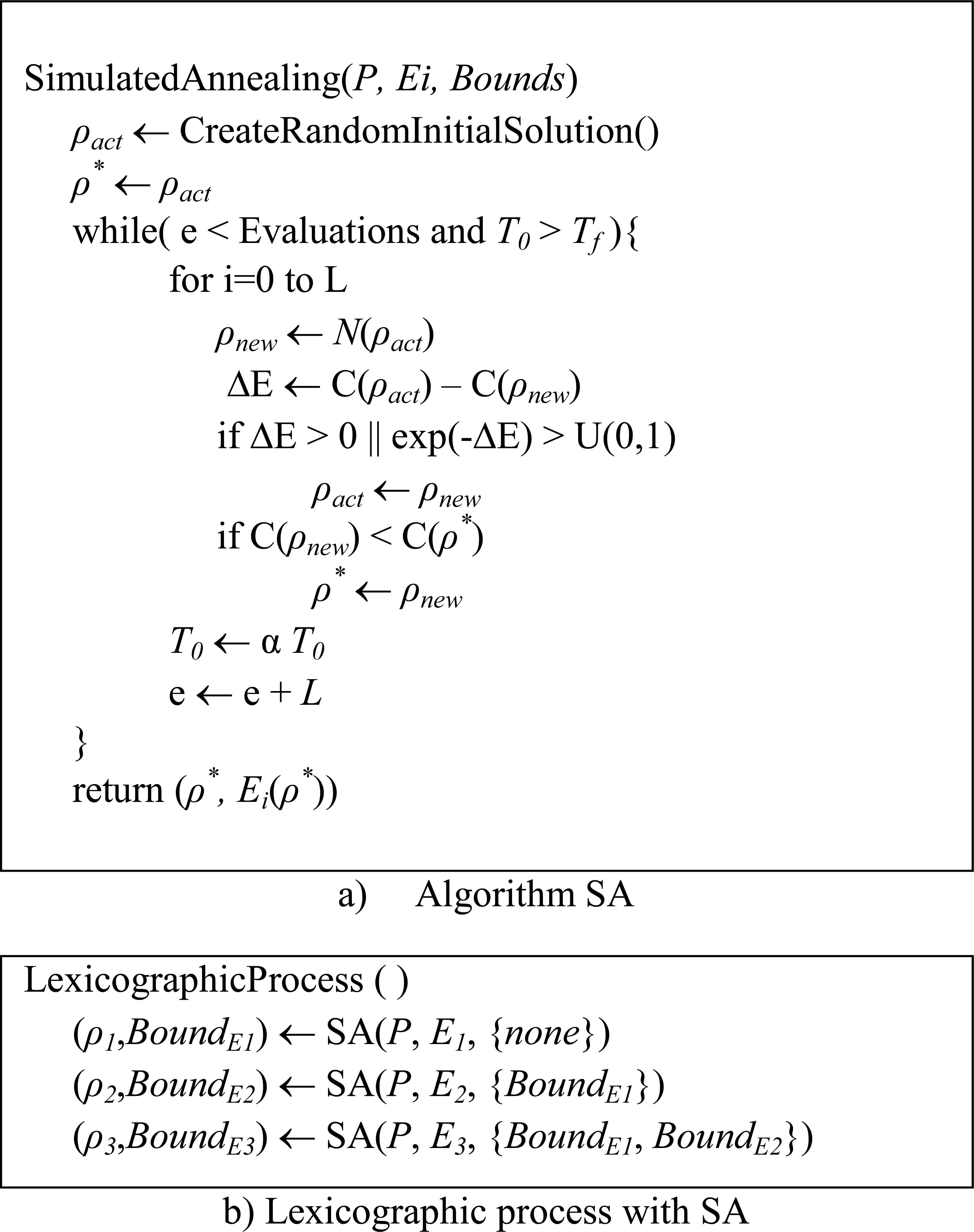
Method for Problem (4) based on SA.
| Possible Values | ||||
|---|---|---|---|---|
| No. | Parameter | V1 | V2 | V3 |
| A | L | 50 | 100 | 200 |
| B | α | 0.85 | 0.95 | 0.98 |
| C | T0 | 1 | 10 | 100 |
| D | Tf | 1x10⁻³ | 1x10⁻⁶ | 1x10⁻⁹ |
| E | Evaluations | 25000 | 50000 | 100000 |
a) Tested Parameter Values
| Parameter Values | |||||
|---|---|---|---|---|---|
| Config. | A | B | C | D | E |
| 1 | 100 | 0.98 | 100 | 1x10⁻⁶ | 100000 |
| 2 | 100 | 0.85 | 10 | 1x10⁻⁶ | 25000 |
| 3 | 50 | 0.85 | 1 | 1x10⁻⁹ | 25000 |
| 4 | 50 | 0.85 | 100 | 1x10⁻³ | 50000 |
| 5 | 200 | 0.95 | 1 | 1x10⁻⁶ | 50000 |
| 6 | 100 | 0.98 | 10 | 1x10⁻⁹ | 50000 |
| 7 | 100 | 0.95 | 1 | 1x10⁻³ | 100000 |
| 8 | 50 | 0.98 | 100 | 1x10⁻⁶ | 100000 |
| 9 | 50 | 0.95 | 10 | 1x10⁻⁹ | 100000 |
| 10 | 200 | 0.95 | 100 | 1x10⁻⁹ | 25000 |
| 11 | 200 | 0.85 | 10 | 1x10⁻⁶ | 100000 |
| 12 | 100 | 0.98 | 1 | 1x10⁻⁹ | 25000 |
| 13 | 200 | 0.98 | 10 | 1x10⁻³ | 25000 |
b) Valid configurations using a CA(13;2,5,3)35
| No. | Parameter | Value |
|---|---|---|
| A | Markov Chain Lengh, L | 100 |
| B | Cooling Factor, α | 0.98 |
| C | Initial Temperature, T0 | 100 |
| D | Final Temperature, Tf | 0.000001 |
| E | Evaluations | 100000 |
c) Best Configuration, Config. 1
Parameters of SA.
The parameters of the SA implementation that required a previous adjustment of their values are: the Markov Chain length L, the cooling factor α, the initial temperature T0, the final temperature Tf, and the stop criterion (as the number of Evaluations). The fine-tuning process followed is the one presented in Section 4.1.2. Table 3a presents the values considered per parameter; Table 3b shows the set of valid configurations tested; and, Table 3c contains the winner configuration through the method, using a random instance. The latter configuration was used to lead the main experimental design proposed in this paper.
4.2. Experimental Design
This section details the experiment conducted to test the performance of the PDA related to the fuzzy outranking relational system proposed in Refs. 3 and 17. The description is divided into in two parts. The first part describes the generation of instances to analyze the Problem (4) formulated to infer model parameters. The second part shows the validation process followed to measure the quality of the estimated parameter values, mainly in its capacity for properly predicting preferences in new sets of instances.
4.2.1 Generating instances
In order to test the model, it was necessary to simulate DM’s responses, and to generate a set of instances as cases of study. For this purpose, we simulate the DM’s preferences through the random generation of the parameter vector η={w,q,p,u,v}, for a given number of criteria, and its combination with one of the considered tuples from (λ,β,ε)={(0.51,0.15,0.07), (0.67,0.15,0.07), (0.70,0.20,0.10), (0.75,0.20,0.10)}. Then, the generated set DMsim-parameters=(η0,λ0,β0,ε0) is considered as the “true” preference parameters of the simulated DM that should be approximated by our inference approach.
Each instance is characterized by: i) a reference set T formed by a finite number of alternatives; and, ii) a set of statements made over pairs (x,y) ∈ T×T, which are given by the DM as its preference judgments. The reference set T is generated using a random function; the number of alternatives, the number of criteria describing each action, and the range of criterion values are defined in advanced for T. In addition, for a particular action, the value of each criterion is generated at random in the specified range. The set A= {P,I,Q,K,R,~,P−1,Q−1,K−1} is the set of preference statements that the real DM establishes on (x,y) ∈ T×T according to Assumption 2. In order to simulate the DM’s responses, we assume that xAiy if xAi(η0,λ0,β0,ε0)y where Ai∈A and Ai(η0,λ0,β0,ε0) is one of the relations given by Definition 1. That is, xAi(η0,λ0,β0,ε0)y is considered as the response from the DM when (s)he is questioned about his/her preference on a pair (x,y).
Given that the work presented in this document searches the identification of algorithms that properly characterizes to a DMsim, it proposes an analysis of their performance on two sets of instances which differ in the number of involved actions. Let’s point out that the use of a different amount of alternatives implies a greater involvement of a DM, reason why these should be taken as small as possible. Due to this reason, the first set (denoted as S10) contains 40 instances where each has a reference set composed by 10 alternatives, and 45 preference statements established using a particular set of preference parameter DMsim-parameters=(η0,λ0,β0,ε0). The second set, referred as S20, is formed by 40 instances each composed by 20 different alternatives, and 190 preference statements established using the same set of preference parameters DMsim-parameters=(η0,λ0,β0,ε0) used in the set S10. The change in the number of alternatives from S10 to S20 allows to study the impact of the number of actions taken into account on the performance of the algorithms.
Each alternative of the sets S10 and S20 is constituted by 10 objectives in this work; and the universe from which these alternatives are formed considers values in the range [1, 10] per objective. Hence, an alternative is generated by randomly assigning a value to each of its 10 objectives.
4.2.2 Validation
In order to validate properly the performance of the considered algorithms GA, PSO, TS, and SA, it is proposed to evaluate and compare the prediction capacity of the best estimation (η*,λ*,β*,ε*) obtained by each them. That prediction capacity can be measured by computing the error achieved on a new set of instances, called S100. For each setting DMsim-parameters=(η0,λ0,β0,ε0) used in generating S10, a validation set V with 100 objects generated at random is created. Each pair (x,y) of V×V is associated with preference statements xAi(η0,λ0,β0,ε0)y and xAj(η*,λ*,β*,ε*)y. Then, in order to evaluate the error existing between a solution to Problem (4) (η*,λ*,β*,ε*) and (η0,λ0,β0,ε0), we propose the use of the indicator defined as in Eq. (5).
Since the objectives in Problem (4) obey a lexicographical order, IP is defined according to the objective E1, which counts inconsistencies derived from the equivalence xP(η0,λ0,β0,ε0)y⇔xP(η*,λ*,β*,ε*)y, for all (x,y)∈V×V. Whenever a tie is produced using the indicator IP, the objectives E2 and E3 of Problem (4) are used to break the tie. Note that the indicator IP is defined as a way of measuring the capacity of prediction, in new instances, of the best estimation (η*,λ*,β*,ε*) obtained for the parameter values.
The new set S100 has 40 instances, each composed by 100 different alternatives, and 4450 preference statements. The best obtained estimations (η*,λ*,β*,ε*) using the set S10 were used to predict the preference relations given in S100, and the resulting preferences were compared against the expected ones, i.e. DMsim-parameters=(η0,λ0,β0,ε0). The previous process is repeated using the set S20.
Finally, the validation process concludes with a summary of the errors obtained per instance and algorithm, in contrast with the DMsim-parameters=(η0,λ0,β0,ε0).
4.3. Results
The results in this section are derived from solving Problem (4), using the proposed method of Section 4.1, under the experimental design presented in Section 4.2. The conducted experiment involves the prediction of the preference statements in a new set of instances S100. It concludes with the results derived from the prediction capacity of the estimated parameter values over the new set of instances. During this experiment, some constraints used in the literature, as in Ref. 20, were considered over the values of the parameters; these constraints are depicted as follows:
- •
wi > 0;
- •
λ > 0.51;
- •
0 ≤ qi ≤ pi < ui < vi(i = 1,···,n);
- •
|(vj + pj)/2 − uj| ≤ 0.1(vj − pj);
Also, this work considers that the DM can provide lower and upper bounds on the values of the parameters. Based on this idea, we include a constraint that establishes the bounds for the parameters values in ±30% of the simulated values.
The content of this section is organized into three parts. The Section 4.3.1 presents a summary of the estimated parameter values obtained using the proposed method, contrasting them with the expected real parameter values. The Section 4.3.2 shows the details of the results concerning the use of the centroids obtained from S10. Finally, the Section 4.3.3 details of the results concerning the use of the centroids obtained from S20.
4.3.1 Estimated parameter values
Given that the algorithms used are nondeterministic, we obtain diverse solutions in the parameter space that hold optimal values. So, it is necessary a strategy that allows an appropriate handling of that diversity, choosing a representative solution.
For this purpose, the centroids (η*,λ*,β*,ε*) are taken as the best estimated values that are returned by the method as a solution for a given instance of Problem (4). In order to obtain a centroid, the method solves 30 times the instance. After that, the sets of solutions reported by the strategy used (i.e. the algorithms GA, PSO, TS, or SA) are put together to form the whole set of solutions.
Finally, the estimated parameter values (ηi,λi,βi,εi) of each solution i, from the whole set of solutions, are summed up individually, to obtain its average. The resulting value of each parameter involved in this process constitutes what is called the centroid.
For space limitation we only show in Table 5 the results of two instances. This table compares the centroids obtained by the algorithms GA, PSO, TS, and SA, against DMsim-parameters=(η0,λ0,β0,ε0), the simulated parameter values. The average percentage of deviation in the instance of S10 is 16% for GA, PSO and TS, and 23% for SA. Besides, these percentages are 16%, 17%, 23% and 22% respectively in the instance of S20. These performances are similar in the other instances.
| Set S10 | Set S20 | |||||||||||||||||||
|---|---|---|---|---|---|---|---|---|---|---|---|---|---|---|---|---|---|---|---|---|
| w1 | w2 | w3 | w4 | w5 | w6 | w7 | w8 | w9 | w10 | w1 | w2 | w3 | w4 | w5 | w6 | w7 | w8 | w9 | w10 | |
| DMsim | 0.09 | 0.12 | 0.10 | 0.08 | 0.09 | 0.11 | 0.09 | 0.09 | 0.10 | 0.10 | 0.09 | 0.12 | 0.10 | 0.08 | 0.09 | 0.11 | 0.09 | 0.09 | 0.10 | 0.10 |
| GA | 0.10 | 0.12 | 0.10 | 0.09 | 0.10 | 0.11 | 0.09 | 0.09 | 0.10 | 0.10 | 0.09 | 0.12 | 0.11 | 0.09 | 0.10 | 0.11 | 0.09 | 0.09 | 0.10 | 0.10 |
| PSO | 0.10 | 0.12 | 0.11 | 0.09 | 0.10 | 0.11 | 0.09 | 0.09 | 0.10 | 0.09 | 0.10 | 0.13 | 0.11 | 0.09 | 0.10 | 0.11 | 0.09 | 0.09 | 0.10 | 0.09 |
| SA | 0.10 | 0.12 | 0.11 | 0.08 | 0.10 | 0.11 | 0.09 | 0.10 | 0.10 | 0.10 | 0.10 | 0.12 | 0.10 | 0.09 | 0.10 | 0.11 | 0.09 | 0.10 | 0.10 | 0.10 |
| TS | 0.10 | 0.12 | 0.10 | 0.09 | 0.10 | 0.11 | 0.09 | 0.10 | 0.10 | 0.10 | 0.10 | 0.12 | 0.10 | 0.09 | 0.10 | 0.11 | 0.09 | 0.10 | 0.10 | 0.10 |
| q1 | q2 | q3 | q4 | q5 | q6 | q7 | q8 | q9 | q10 | q1 | q2 | q3 | q4 | q5 | q6 | q7 | q8 | q9 | q10 | |
| DMsim | 0.15 | 0.17 | 0.15 | 0.13 | 0.15 | 0.13 | 0.13 | 0.16 | 0.13 | 0.12 | 0.15 | 0.17 | 0.15 | 0.13 | 0.15 | 0.13 | 0.13 | 0.16 | 0.13 | 0.12 |
| GA | 0.16 | 0.17 | 0.15 | 0.14 | 0.16 | 0.12 | 0.13 | 0.17 | 0.13 | 0.12 | 0.16 | 0.17 | 0.15 | 0.13 | 0.16 | 0.13 | 0.13 | 0.16 | 0.13 | 0.13 |
| PSO | 0.16 | 0.17 | 0.16 | 0.14 | 0.17 | 0.14 | 0.14 | 0.16 | 0.13 | 0.13 | 0.16 | 0.18 | 0.17 | 0.13 | 0.16 | 0.13 | 0.13 | 0.17 | 0.14 | 0.12 |
| SA | 0.17 | 0.19 | 0.17 | 0.16 | 0.18 | 0.15 | 0.14 | 0.18 | 0.14 | 0.14 | 0.18 | 0.17 | 0.16 | 0.14 | 0.17 | 0.13 | 0.14 | 0.18 | 0.14 | 0.13 |
| TS | 0.17 | 0.18 | 0.17 | 0.14 | 0.17 | 0.14 | 0.14 | 0.18 | 0.14 | 0.13 | 0.19 | 0.19 | 0.19 | 0.16 | 0.18 | 0.15 | 0.16 | 0.19 | 0.15 | 0.14 |
| p1 | p2 | p3 | p4 | p5 | p6 | p7 | p8 | p9 | p10 | p1 | p2 | p3 | p4 | p5 | p6 | p7 | p8 | p9 | p10 | |
| DMsim | 0.70 | 0.65 | 0.62 | 0.66 | 0.71 | 0.61 | 0.66 | 0.73 | 0.74 | 0.70 | 0.70 | 0.65 | 0.62 | 0.66 | 0.71 | 0.61 | 0.66 | 0.73 | 0.74 | 0.70 |
| GA | 0.65 | 0.63 | 0.53 | 0.60 | 0.67 | 0.54 | 0.57 | 0.68 | 0.68 | 0.62 | 0.62 | 0.68 | 0.56 | 0.62 | 0.65 | 0.53 | 0.55 | 0.68 | 0.67 | 0.65 |
| PSO | 0.71 | 0.65 | 0.61 | 0.65 | 0.70 | 0.62 | 0.64 | 0.75 | 0.71 | 0.71 | 0.69 | 0.65 | 0.64 | 0.65 | 0.71 | 0.61 | 0.67 | 0.71 | 0.74 | 0.71 |
| SA | 0.82 | 0.72 | 0.69 | 0.71 | 0.79 | 0.63 | 0.72 | 0.84 | 0.82 | 0.72 | 0.75 | 0.67 | 0.67 | 0.71 | 0.74 | 0.63 | 0.68 | 0.78 | 0.81 | 0.76 |
| TS | 0.78 | 0.70 | 0.68 | 0.74 | 0.80 | 0.68 | 0.74 | 0.82 | 0.82 | 0.79 | 0.82 | 0.77 | 0.70 | 0.74 | 0.79 | 0.68 | 0.75 | 0.84 | 0.82 | 0.81 |
| u1 | u2 | u3 | u4 | u5 | u6 | u7 | u8 | u9 | u10 | u1 | u2 | u3 | u4 | u5 | u6 | u7 | u8 | u9 | u10 | |
| DMsim | 1.66 | 1.89 | 1.67 | 1.63 | 1.56 | 1.65 | 1.52 | 1.69 | 1.55 | 1.76 | 1.66 | 1.89 | 1.67 | 1.63 | 1.56 | 1.65 | 1.52 | 1.69 | 1.55 | 1.76 |
| GA | 1.92 | 1.99 | 2.01 | 1.88 | 1.87 | 1.99 | 1.92 | 1.94 | 1.79 | 1.99 | 1.84 | 2.08 | 1.97 | 1.87 | 1.84 | 1.94 | 1.90 | 1.91 | 1.77 | 2.04 |
| PSO | 1.82 | 2.09 | 1.93 | 1.83 | 1.77 | 1.91 | 1.76 | 1.86 | 1.75 | 2.00 | 1.85 | 2.01 | 1.92 | 1.80 | 1.81 | 1.91 | 1.80 | 1.85 | 1.73 | 1.99 |
| SA | 2.31 | 2.22 | 2.61 | 2.23 | 2.33 | 2.39 | 2.56 | 2.24 | 2.10 | 2.45 | 2.10 | 2.11 | 2.34 | 2.13 | 2.11 | 2.31 | 2.28 | 2.07 | 2.08 | 2.41 |
| TS | 2.18 | 2.11 | 2.38 | 2.15 | 2.16 | 2.37 | 2.44 | 2.16 | 2.03 | 2.39 | 2.10 | 2.18 | 2.31 | 2.12 | 2.10 | 2.25 | 2.26 | 2.13 | 1.93 | 2.30 |
| v1 | v2 | v3 | v4 | v5 | v6 | v7 | v8 | v9 | v10 | v1 | v2 | v3 | v4 | v5 | v6 | v7 | v8 | v9 | v10 | |
| DMsim | 3.98 | 3.67 | 4.69 | 3.97 | 4.13 | 4.67 | 4.75 | 3.86 | 3.66 | 4.41 | 3.98 | 3.67 | 4.69 | 3.97 | 4.13 | 4.67 | 4.75 | 3.86 | 3.66 | 4.41 |
| GA | 3.28 | 3.41 | 3.75 | 3.25 | 3.25 | 3.59 | 3.53 | 3.30 | 2.95 | 3.56 | 3.22 | 3.48 | 3.66 | 3.22 | 3.21 | 3.55 | 3.54 | 3.21 | 2.97 | 3.69 |
| PSO | 3.47 | 3.65 | 3.93 | 3.49 | 3.53 | 3.92 | 3.83 | 3.41 | 3.24 | 3.92 | 3.65 | 3.53 | 3.98 | 3.55 | 3.54 | 4.00 | 3.82 | 3.44 | 3.25 | 3.84 |
| SA | 4.14 | 3.98 | 4.94 | 4.09 | 4.27 | 4.53 | 4.86 | 3.95 | 3.67 | 4.54 | 3.69 | 3.72 | 4.29 | 3.80 | 3.79 | 4.29 | 4.22 | 3.52 | 3.73 | 4.35 |
| TS | 3.87 | 3.68 | 4.43 | 3.88 | 3.90 | 4.42 | 4.64 | 3.79 | 3.57 | 4.28 | 3.56 | 3.74 | 4.27 | 3.71 | 3.69 | 4.06 | 4.09 | 3.64 | 3.25 | 4.04 |
| λ | β | ε | λ | β | ε | |||||||||||||||
| DMsim | 0.66 | 0.18 | 0.09 | 0.66 | 0.18 | 0.09 | ||||||||||||||
| GA | 0.69 | 0.18 | 0.09 | 0.68 | 0.17 | 0.09 | ||||||||||||||
| PSO | 0.66 | 0.18 | 0.09 | 0.67 | 0.18 | 0.09 | ||||||||||||||
| SA | 0.74 | 0.20 | 0.09 | 0.74 | 0.19 | 0.09 | ||||||||||||||
| TS | 0.70 | 0.19 | 0.09 | 0.72 | 0.21 | 0.10 | ||||||||||||||
Comparison of average estimated parameter values of each algorithm against the average parameter values of a DMsim per set of instances S10 and S20.
Table 6 shows the average of the estimated parameter values for all the instances in the sets S10 and S20. This table provides the average of the simulated parameter values, DMsim-parameters=(η0,λ0,β0,ε0), and the average of the centroids (η*,λ*,β*,ε*) obtained using the algorithms GA, PSO, TS, and SA.
| Instance 39 of set S10 | Instance 38 of set S20 | |||||||||||||||||||
|---|---|---|---|---|---|---|---|---|---|---|---|---|---|---|---|---|---|---|---|---|
| w1 | w2 | w3 | w4 | w5 | w6 | w7 | w8 | w9 | w10 | w1 | w2 | w3 | w4 | w5 | w6 | w7 | w8 | w9 | w10 | |
| DMsim | 0.12 | 0.12 | 0.12 | 0.09 | 0.10 | 0.09 | 0.09 | 0.08 | 0.09 | 0.06 | 0.07 | 0.11 | 0.11 | 0.07 | 0.08 | 0.09 | 0.07 | 0.10 | 0.11 | 0.15 |
| GA | 0.12 | 0.11 | 0.13 | 0.11 | 0.11 | 0.11 | 0.11 | 0.06 | 0.08 | 0.06 | 0.05 | 0.10 | 0.08 | 0.08 | 0.11 | 0.10 | 0.08 | 0.10 | 0.11 | 0.19 |
| PSO | 0.15 | 0.16 | 0.12 | 0.09 | 0.09 | 0.09 | 0.11 | 0.09 | 0.11 | 0.01 | 0.09 | 0.13 | 0.11 | 0.08 | 0.10 | 0.12 | 0.09 | 0.08 | 0.13 | 0.08 |
| SA | 0.12 | 0.13 | 0.13 | 0.09 | 0.10 | 0.10 | 0.12 | 0.08 | 0.09 | 0.05 | 0.08 | 0.13 | 0.08 | 0.07 | 0.07 | 0.10 | 0.08 | 0.11 | 0.12 | 0.17 |
| TS | 0.12 | 0.13 | 0.11 | 0.08 | 0.11 | 0.09 | 0.10 | 0.09 | 0.09 | 0.08 | 0.07 | 0.13 | 0.13 | 0.08 | 0.07 | 0.11 | 0.07 | 0.10 | 0.09 | 0.16 |
| q1 | q2 | q3 | q4 | q5 | q6 | q7 | q8 | q9 | q10 | q1 | q2 | q3 | q4 | q5 | q6 | q7 | q8 | q9 | q10 | |
| DMsim | 0.19 | 0.18 | 0.13 | 0.10 | 0.12 | 0.10 | 0.13 | 0.18 | 0.11 | 0.10 | 0.14 | 0.16 | 0.18 | 0.12 | 0.18 | 0.12 | 0.12 | 0.16 | 0.11 | 0.16 |
| GA | 0.19 | 0.20 | 0.17 | 0.12 | 0.10 | 0.12 | 0.15 | 0.23 | 0.08 | 0.08 | 0.15 | 0.19 | 0.17 | 0.09 | 0.17 | 0.09 | 0.13 | 0.18 | 0.11 | 0.11 |
| PSO | 0.16 | 0.21 | 0.13 | 0.12 | 0.13 | 0.12 | 0.10 | 0.17 | 0.11 | 0.10 | 0.13 | 0.21 | 0.16 | 0.13 | 0.18 | 0.11 | 0.13 | 0.17 | 0.09 | 0.18 |
| SA | 0.23 | 0.23 | 0.17 | 0.14 | 0.16 | 0.11 | 0.17 | 0.24 | 0.12 | 0.11 | 0.16 | 0.22 | 0.23 | 0.15 | 0.21 | 0.12 | 0.12 | 0.20 | 0.13 | 0.20 |
| TS | 0.21 | 0.18 | 0.14 | 0.13 | 0.13 | 0.12 | 0.12 | 0.20 | 0.14 | 0.11 | 0.16 | 0.20 | 0.23 | 0.15 | 0.15 | 0.09 | 0.15 | 0.15 | 0.15 | 0.20 |
| p1 | p2 | p3 | p4 | p5 | p6 | p7 | p8 | p9 | p10 | p1 | p2 | p3 | p4 | p5 | p6 | p7 | p8 | p9 | p10 | |
| DMsim | 0.76 | 0.87 | 0.56 | 0.74 | 0.55 | 0.49 | 0.66 | 0.83 | 0.62 | 0.75 | 0.88 | 0.50 | 0.56 | 0.68 | 0.86 | 0.69 | 0.55 | 0.49 | 0.81 | 0.68 |
| GA | 0.96 | 0.74 | 0.52 | 0.56 | 0.55 | 0.42 | 0.47 | 0.79 | 0.52 | 0.54 | 0.62 | 0.47 | 0.40 | 0.53 | 0.68 | 0.74 | 0.39 | 0.55 | 0.70 | 0.69 |
| PSO | 0.74 | 0.97 | 0.57 | 0.85 | 0.54 | 0.50 | 0.76 | 0.93 | 0.51 | 0.64 | 1.00 | 0.43 | 0.73 | 0.66 | 0.66 | 0.48 | 0.50 | 0.61 | 0.81 | 0.53 |
| SA | 0.62 | 0.67 | 0.50 | 0.79 | 0.69 | 0.42 | 0.80 | 1.08 | 0.60 | 0.93 | 0.98 | 0.47 | 0.52 | 0.87 | 1.01 | 0.85 | 0.69 | 0.39 | 1.05 | 0.84 |
| TS | 0.93 | 0.95 | 0.60 | 0.92 | 0.58 | 0.61 | 0.71 | 0.90 | 0.67 | 0.80 | 1.11 | 0.60 | 0.71 | 0.88 | 1.13 | 0.89 | 0.64 | 0.63 | 1.04 | 0.52 |
| u1 | u2 | u3 | u4 | u5 | u6 | u7 | u8 | u9 | u10 | u1 | u2 | u3 | u4 | u5 | u6 | u7 | u8 | u9 | u10 | |
| DMsim | 1.47 | 1.71 | 1.59 | 1.25 | 1.58 | 1.63 | 1.28 | 1.64 | 1.26 | 2.03 | 1.63 | 2.00 | 1.39 | 1.69 | 1.26 | 1.74 | 1.58 | 1.44 | 1.96 | 2.00 |
| GA | 1.61 | 2.06 | 2 | 1.61 | 2.02 | 1.65 | 1.67 | 1.85 | 1.59 | 2.11 | 1.94 | 2.15 | 1.81 | 1.81 | 1.47 | 2.00 | 1.92 | 1.61 | 1.97 | 1.94 |
| PSO | 1.78 | 2.01 | 2.02 | 1.35 | 1.88 | 1.9 | 1.67 | 1.49 | 1.62 | 1.88 | 2.07 | 2.38 | 1.80 | 1.89 | 1.54 | 2.03 | 1.83 | 1.62 | 2.55 | 2.34 |
| SA | 2.22 | 2.09 | 2.77 | 2.6 | 2.72 | 2.12 | 1.93 | 1.89 | 2.13 | 2.34 | 3.15 | 2.04 | 2.90 | 2.72 | 1.80 | 2.29 | 2.55 | 1.87 | 2.43 | 2.66 |
| TS | 2.13 | 2.06 | 2.32 | 2.35 | 2.5 | 2.05 | 2.24 | 1.87 | 1.85 | 2.43 | 2.88 | 2.58 | 2.30 | 2.55 | 1.95 | 2.64 | 2.06 | 1.88 | 1.90 | 2.60 |
| v1 | v2 | v3 | v4 | v5 | v6 | v7 | v8 | v9 | v10 | v1 | v2 | v3 | v4 | v5 | v6 | v7 | v8 | v9 | v10 | |
| DMsim | 3.53 | 3.12 | 5.29 | 3.95 | 5.15 | 3.63 | 4.91 | 3.04 | 3.28 | 3.88 | 5.13 | 4.84 | 5.52 | 4.11 | 3.23 | 4.78 | 5.51 | 3.99 | 4.09 | 4.13 |
| GA | 2.55 | 3.6 | 3.84 | 2.88 | 3.87 | 3.03 | 3.44 | 3.15 | 2.97 | 3.85 | 3.62 | 3.76 | 3.87 | 3.34 | 2.41 | 3.36 | 3.86 | 2.82 | 3.46 | 3.56 |
| PSO | 3.41 | 3.45 | 3.97 | 2.6 | 3.6 | 4.64 | 3.41 | 2.27 | 2.88 | 3.56 | 4.81 | 3.83 | 4.26 | 3.27 | 2.45 | 5.27 | 4.22 | 3.33 | 4.88 | 3.84 |
| SA | 4.23 | 3.98 | 5.65 | 4.99 | 5.34 | 4.29 | 3.49 | 2.47 | 4.12 | 3.32 | 5.97 | 3.51 | 5.84 | 5.18 | 3.00 | 3.52 | 4.97 | 3.15 | 4.35 | 5.07 |
| TS | 3.77 | 3.13 | 4.57 | 4.3 | 4.98 | 3.5 | 4.26 | 2.92 | 3.39 | 4.34 | 4.19 | 4.57 | 4.39 | 4.78 | 3.20 | 4.98 | 3.94 | 3.22 | 3.08 | 5.12 |
| λ | β | ε | λ | β | ε | |||||||||||||||
| DMsim | 0.70 | 0.20 | 0.10 | 0.67 | 0.15 | 0.07 | ||||||||||||||
| GA | 0.71 | 0.17 | 0.11 | 0.67 | 0.15 | 0.07 | ||||||||||||||
| PSO | 0.80 | 0.19 | 0.10 | 0.62 | 0.14 | 0.06 | ||||||||||||||
| SA | 0.74 | 0.21 | 0.13 | 0.78 | 0.14 | 0.08 | ||||||||||||||
| TS | 0.76 | 0.21 | 0.11 | 0.85 | 0.19 | 0.07 | ||||||||||||||
Estimated parameter values for instances I39 of set S10 and I38 of set S20.
4.3.2 Performance of prediction of centroids from S10 over the new set S100
In this part of the experiment, the centroids (η*, λ*,β*,ε*) were computed under the method proposed in Section 4.1, and having as input the set of instances S10. The centroids are used to predict the preference statements xA(η0,λ0,β0,ε0)y and yA(η0,λ0,β0,ε0)x for every pair (x,y) ∈ V×V, where V is the test set formed in each instance of S100. The maximum number of inconsistencies that can be found in an instance is 9900, because each of the 4450 judgments of the DMsim is evaluated as xAy and yAx.
Table 7 summarizes the results from the validation process described in Section 4.2.3. An instance in this table is represented by a row, and a set of columns named after one of the tuples (λ,β,ε)={(0.51,0.15,0.07), (0.67,0.15,0.07), (0.70,0.20,0.10), (0.75, 0.20, 0.10)}. Each instance has associated four cells in the table, which contain the value of IP, i.e. the number of inconsistencies obtained by the algorithms GA, PSO, TS, and SA. Note that the only preference relation under study was the strict preference P, and it was enough to rank the algorithms properly. These results were statistically validated. Firstly, using the Friedman test with a significance level of 0.05 it was found that significant differences exist among the algorithms; secondly, the Finner test indicated the superiority of GA over SA and TS.
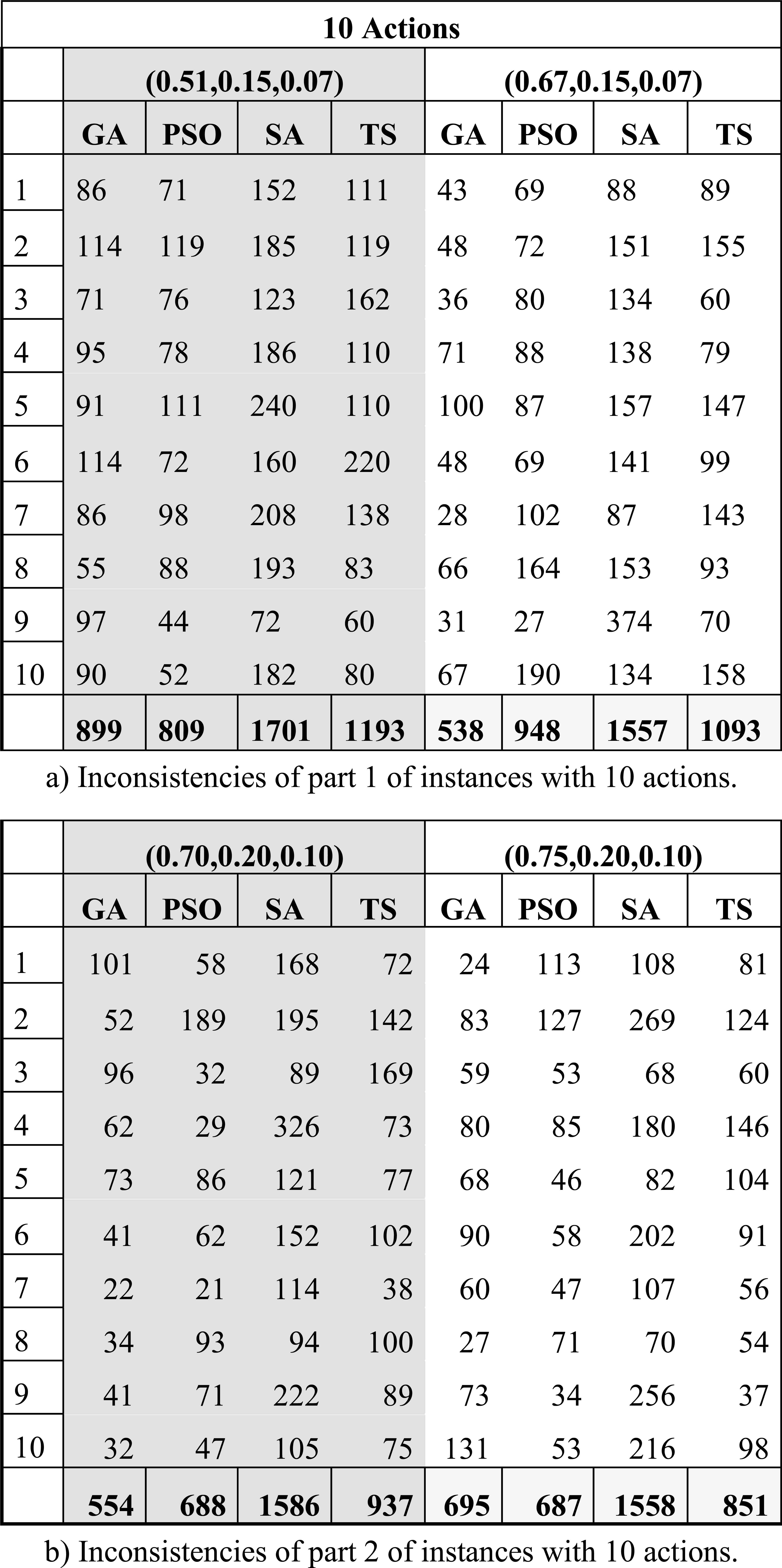
Summary of the indicator IP from results derived from set S100 using centroids derived from set S10.
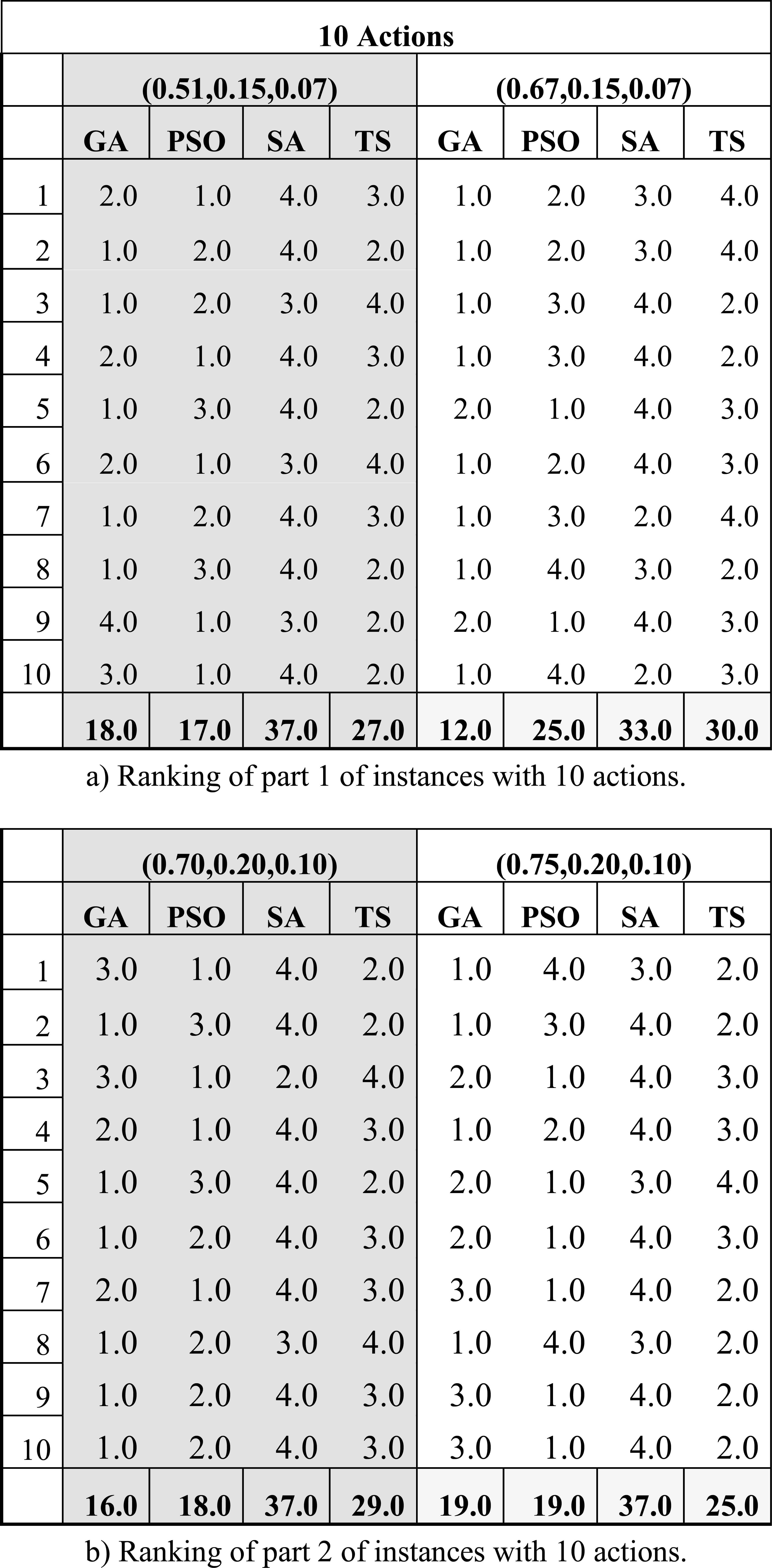
Table 8 shows the rank of the algorithms GA, PSO, SA, TS, according to the value of indicator IP shown in Table 7, which evaluates the most important preference relation for this study. Each row of Table 8 is combined with a tuple from (λ,β,ε), i.e. a group of four columns with such title, to represent an instance of the set S10. The algorithms are ranked per instance, the one with the minimum number of inconsistencies (or incorrect judgments) is ranked 1, the next one 2, and so on.
Ranking of the performance of the algorithms per instance, when the centroids obtained from S10 are validated using S100.
Table 9 shows the Borda score of the ranks obtained by each algorithm in Table 8; Figure 7 compares the ranks graphically (grouped by tuples). Using each of the four groups of configurations presented in Table 7, several statistical tests were developed to validate the performance of the algorithms.
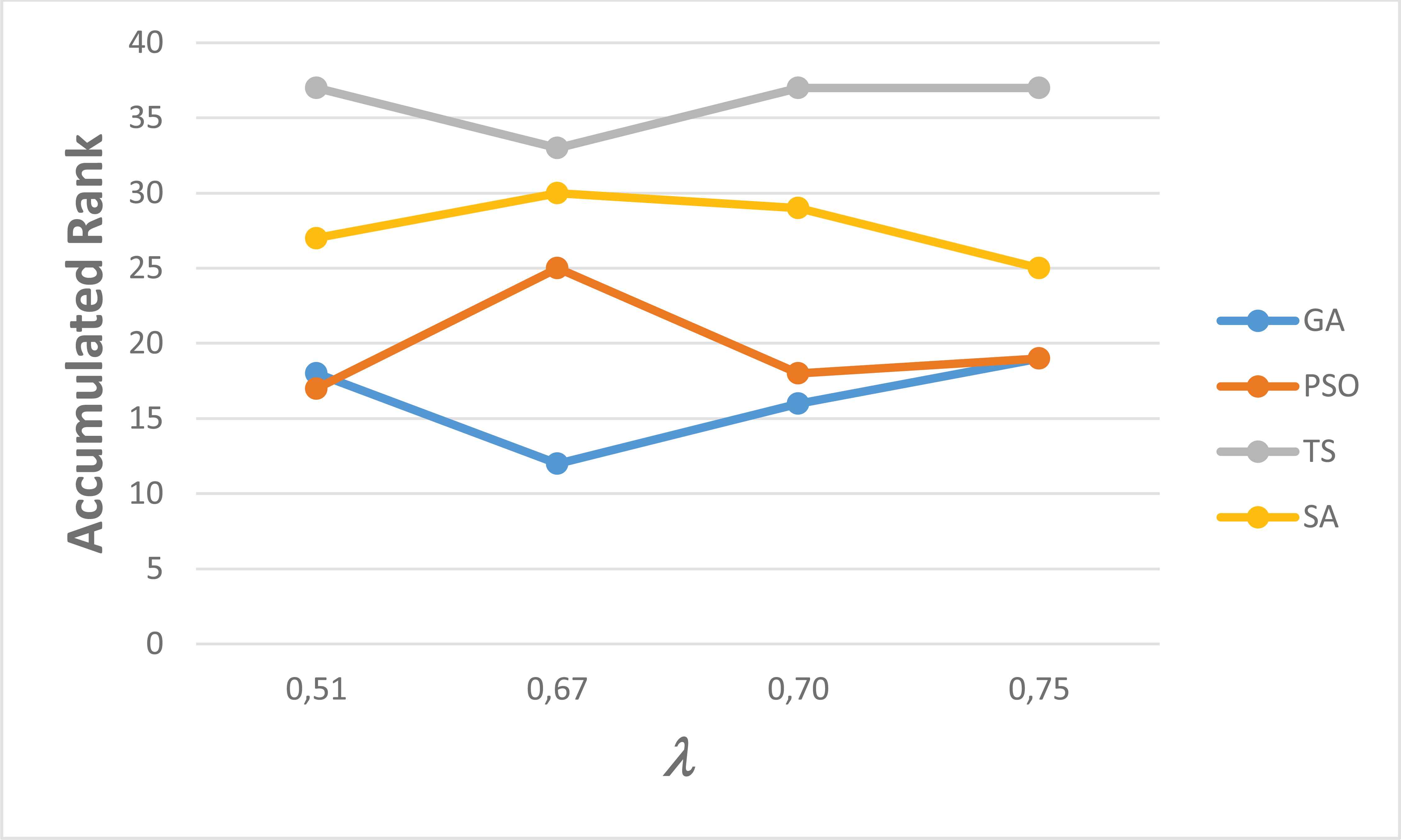
Performance of prediction of the centroids obtained per algorithm using the set S10 over the set S100 using: a) an accumulated sum of ranks; and, b) a graph of ranks per value λ. Note that each value λ is associated with particular values of (β,ε), as indicated in Table 7.
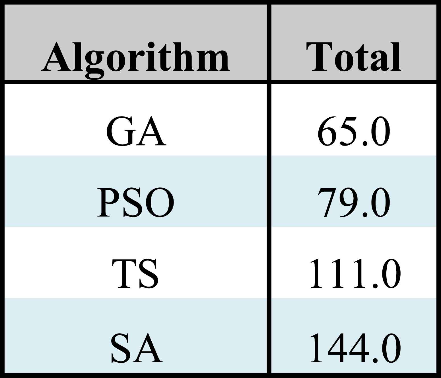
Borda score from Table 8.
Summing up the information presented in this section, the centroids obtained using the GA statistically obtained a performance at least similar to the remaining algorithms, but they minimized the total number of inconsistencies found among all the instances (it achieved 2686 according to Table 7). Also, the GA results yielded the minimum number of inconsistencies in 23 of the 40 instances (see Table 8) reaching the best Borda score. Finally, if we take into account that the centroids resulting from this metaheuristic had also previously shown a good performance in estimating the parameter values of the preference model, then we can conclude that it has the best performance using only 10 alternatives.
4.3.3 Performance of prediction of centroids from S20 over the new set S100
In this part of the experiment, the centroids were computed under the method proposed in Section 4.1, and having as input the set of instances S20.
Similarly to Table 8, Table 10 summarizes the results from the validation process described in Section 4.2.3. Again, when validating these results with the Friedman test (and a significance level of 0.05), there were significant differences among the algorithms. Also, with the use of the Finner test it was found a superiority of GA over SA and TS. Besides, the Wilcoxon test, with a p-value of 0.008, finds significant differences between GA and PSO.
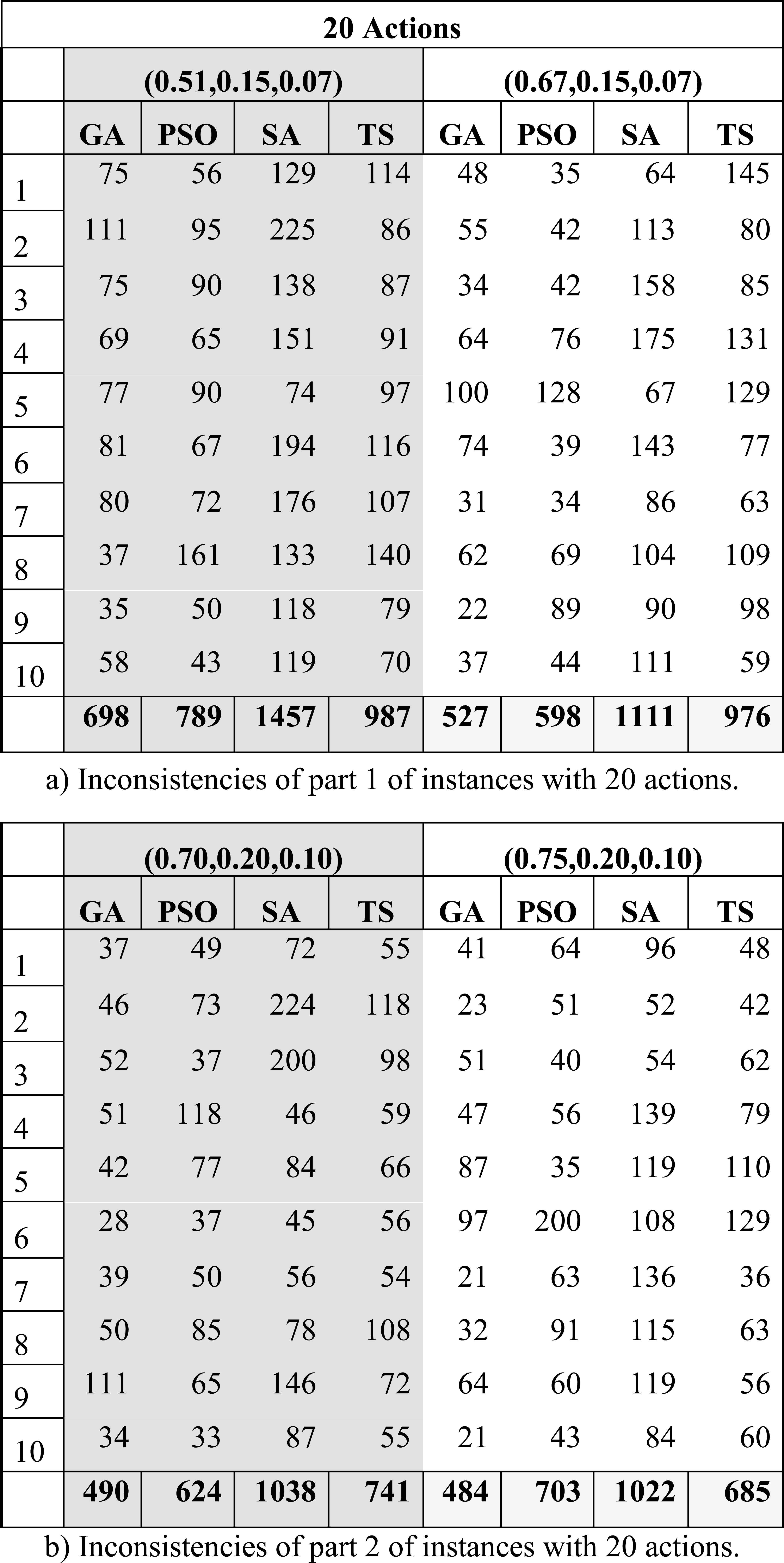
Summary of the indicator IP with results derived from the set S100 using centroids derived from the set S20.
Table 12 shows a summary of the ranks obtained by each algorithm in Table 11. Figure 8 groups the ranks per tuple, and graphically compares them, supporting the conclusion that the best algorithm is indeed GA.
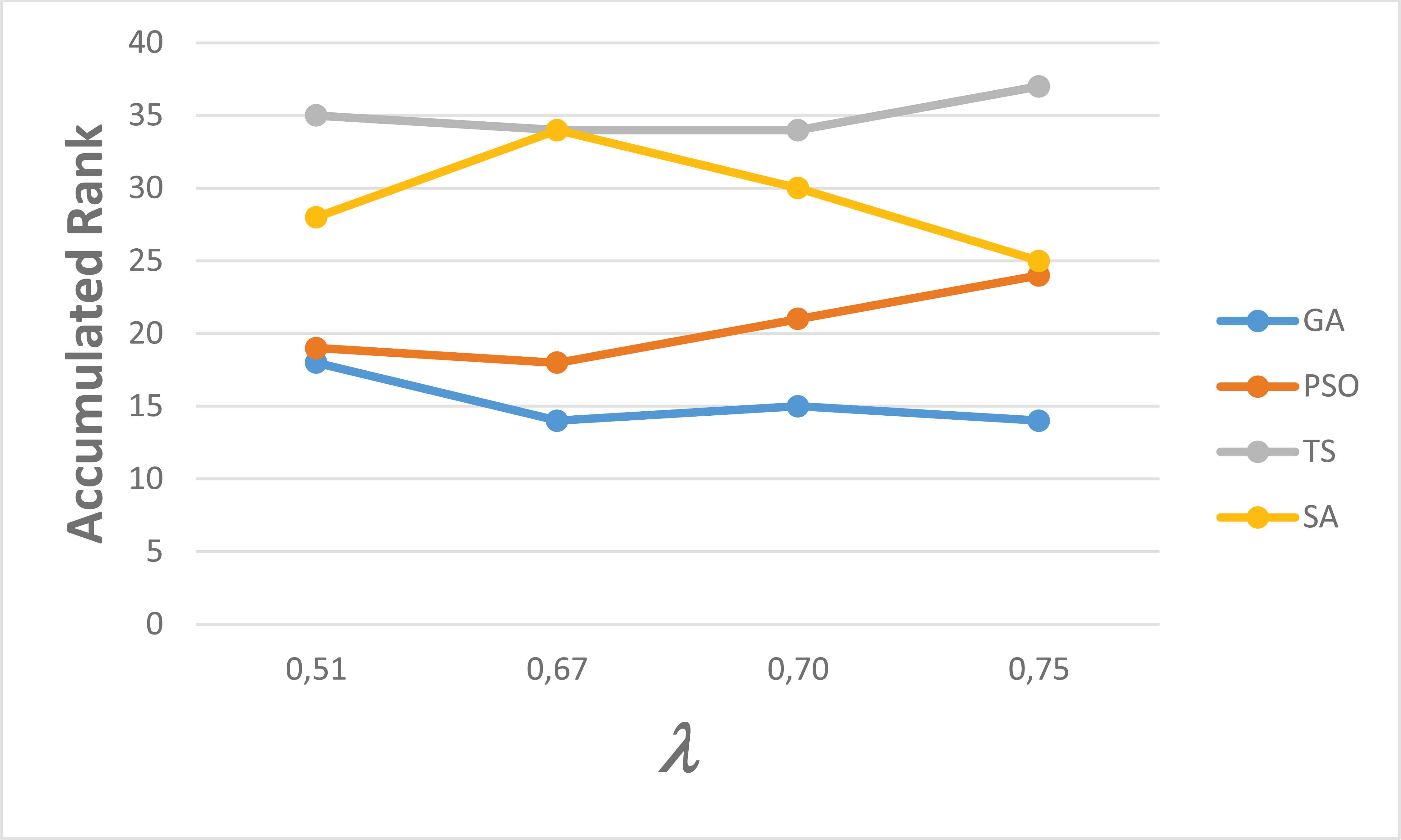
Performance of prediction of the centroids obtained by each algorithm using S20 over the set S100 using: a) an accumulated sum of ranks; and, b) a graph of ranks per value λ. Note that each value λ is associated with particular values of (β,ε), as indicated in Table 7.
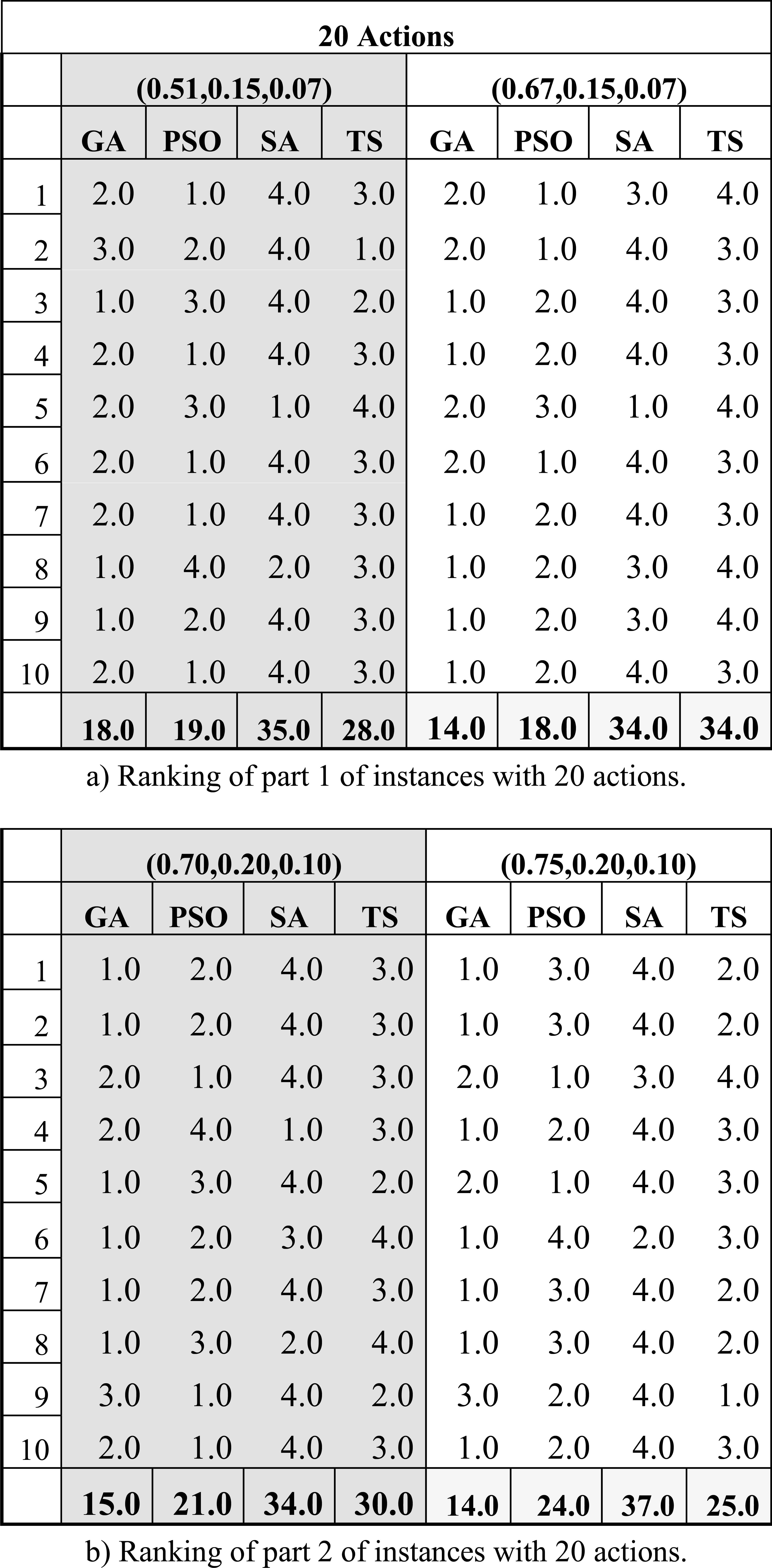
Ranking of the performance of the algorithms per instance, when the centroids obtained from S20 are validated using S100.
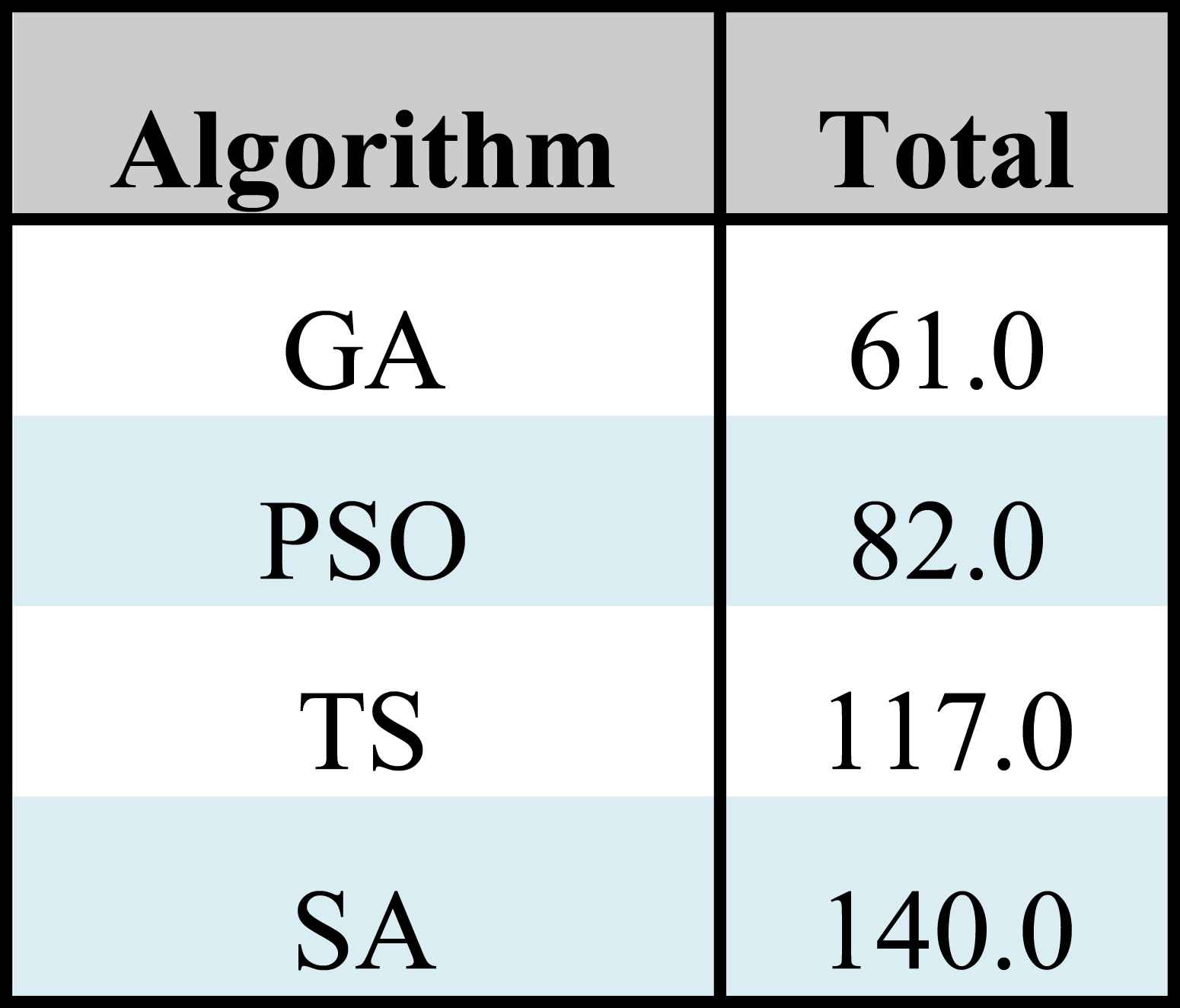
Borda score from Table 11.
4.4. Discussion
The model proposed was tested under an experimental design involving two different sets of instances. The set S10 involved 40 instances, each having 10 actions and all the possible preferences established among them, which means a total of 45 judgments that should be made by the DM that is being modeled. The set S20 also involved 10 instances, but in this case each having 20 actions and a total of 190 judgments that should be made by the DM. On the set S10, using GA, we obtained only 2686 inconsistencies on the 396,000 strict preference simulated statements counted over all the set of instances from the test set S100. It means a 0.68% of error. On the other hand, the use of the set S20 combined with GA reduced the error to 0.55%. Although the results were improved by using a greater set of actions, the cognitive effort that it implies for the DM may be not justified; i.e., the increment of more than 400% in the amount of judgments that the DM must provide is probably not justified by a relatively weak improvement in the reduction of the number of inconsistencies. So, the DM-decision analyst couple should find a compromise between the model accuracy and the required cognitive effort.
In addition, and according to all the results already presented, it is considered that the best algorithm is GA, because it has the best rank value, i.e. it minimizes the inconsistencies in most instances. Further, the performance on the estimation of parameter values through the use of GA on the instances can be considered adequate because: a) it uses a small number of DM’s judgments; b) it ranks better among all the algorithms; and, c) its superiority was proved through statistical tests.
5. Concluding Remarks
This work proposes an approach based on a Preference Disaggregation Analysis procedure to infer parameter settings for the model of preferences proposed by Fernandez3. The preference model is based on outranking relations which require the use of weights and thresholds parameters, denoted by (η,λ), and some additional symmetric and asymmetric parameters (β,ε). The relations involved are of strict preference, indifference, weak preference, incomparability, K-preference, and non-preference. The model of preferences under study has not been addressed by a PDA methodology before. The proposed PDA strategy involves an optimization model for the indirect parameter setting, and its solution using a method based on meta-heuristics.
The optimization model, called Problem (4), is an optimization problem that approximates the values of the parameters (η,λ,β,ε) through the minimization of the inconsistencies found between the preference statements produced by estimated parameter values, and preference judgments established by a Decision Maker (DM) through a reference set. This problem is based in three lexicographically ordered objectives. The most important objective relates the inconsistencies from the strict preference relation. The second objective in importance involves the combined inconsistencies from the indifference and weak preference relations. The third objective incorporates the inconsistencies found in the remaining relations.
The performance of the proposed PDA procedure was tested using four different algorithms: Genetic Algorithm (GA), Particle Swarm Optimization (PSO), Tabu Search (TS), and Simulated Annealing (SA). The experimental design used to test their performance involves the estimation of the parameters (η,λ,β,ε) in two different set of instances formed by small size reference sets. The quality of the best estimated parameters, called centroids, was evaluated by determining both: a) the percentage of deviation of the estimated parameters, and the expected ones; and, b) the number of inconsistencies obtained when using the estimated parameters in the prediction of preference relations on new outcomes, i.e. a new set of instances.
The results reveal that the algorithms GA and PSO had the best performance in relation with the percentage of deviation, because of their reductions in the gap between estimated and simulated parameter values of up to a 16% of deviation in the instances considered. However, the algorithm GA had the best quality in the prediction of preferences in new outcomes, or instances, having the minimum number of inconsistencies in more than 50% of the instances, in comparison with the other approaches. Also, it was revealed that our proposal requires a relatively small number of judgments defined by a DM to properly estimate parameter values that yield a minimal number of inconsistencies in new outcomes.
Acknowledgements
This work has been partially supported by PRODEP and the following projects: a) CONACYT Project 236154, b) Project 3058 from the program Cátedras CONACyT, and c) Project 269890 from CONACYT networks.
Appendix A. Calculus of the degree of credibility of outranking σ(x,y)
The ELECTRE methods introduced a binary relation S based on xSy. Proposition xSy (‘x outranks y’) holds if, and only if, the DM has sufficient arguments in favor of ‘x is at least as good as y’ and there are no strong arguments against it. In more formal way, the coalition of the criteria G in agreement with that proposition is strong enough, and there is no important coalition discordant with it, see Ref. 16. This can be expressed by the following logical equivalence40:
- a)
C(x,y) is the predicate about the strength of the concordance coalition; this coalition is composed of two criterion subsets :
- •
C(xSy) = {gj ∈G such that gj(x) - gj(y) ≥-qj};
- •
C(yQx) = {gj ∈G such that gj(y) -pj ≤ gj(x) < gj(y) -qj} (Q denotes ‘weak preference’);
- •
pj and qj denote the preference and indifference thresholds for criterion j (pj ≥qj ≥0).
- •
- b)
D(x,y) is the predicate about the strength of the discordance coalition C(yPx) = {j ∈G such that gj(y) - gj(x) ≥pj }(P denotes ‘strict preference’)
- c)
∧ and ~ are the logical connectives for fuzzy conjunction and fuzzy negation, respectively.
Let c(x,y) denote the truth degree of predicate C(x,y). Using the ‘product’ operator for conjunction, in ELECTRE III the degree of credibility of xSy is calculated by:
The concordance index c(x,y) is defined as follows:
The partial discordance is measured in comparison with a veto threshold vj, which is the maximum difference gj(y) - gj(x) compatible with σ(x,y) > 0. Following Mousseau and Dias in Ref. 32, we shall use a simplification of the original formulation of the discordance indices in the ELECTRE III method given by:
σ(x,y) is calculated by combining Eqs. A.1–A.5 with Eq. (5).
References
Cite this article
TY  - JOUR
AU  - Laura Cruz-Reyes
AU  - Eduardo Fernandez
AU  - Nelson Rangel-Valdez
PY  - 2017
DA  - 2017/01/01
TI  - A metaheuristic optimization-based indirect elicitation of preference parameters for solving many-objective problems
JO  - International Journal of Computational Intelligence Systems
SP  - 56
EP  - 77
VL  - 10
IS  - 1
SN  - 1875-6883
UR  - https://doi.org/10.2991/ijcis.2017.10.1.5
DO  - 10.2991/ijcis.2017.10.1.5
ID  - Cruz-Reyes2017
ER  -