
Fault Diagnosis of Bearings Using an Intelligence-Based Autoregressive Learning Lyapunov Algorithm
 , Jong-Myon Kim2, *,
 - DOI
- 10.2991/ijcis.d.201228.002How to use a DOI?
- Keywords
- Lyapunov-based observer; Fuzzy algorithm; Adaptive technique; Autoregressive learning signal modeling; Support vector regression; Support vector machine; Fault diagnosis
- Abstract
Bearings are complex components with nonlinear behavior that are used to reduce the effect of inertia. They are used in applications such as induction motors and rotating components. Condition monitoring and effective data analysis are important aspects of fault detection and classification in bearings. Thus, an effective and robust hybrid technique for fault detection and identification is presented in this study. The proposed scheme has four main steps. First, a mathematical approach is combined with an autoregressive learning technique to approximate the vibration signal under normal conditions and extract the state-space equation. In the next step, an intelligence-based observer is designed using a combination of the robust Lyapunov-based method, autoregressive learning scheme, fuzzy technique, and adaptive algorithm. The intelligence-based observer is the main part of the algorithm that determines the fault estimation in the bearing. After estimating the signals, in the third step, the residual signals are generated, resampled, and the root mean square (RMS) is extracted from the resampled residual signals. Then, in the final step, the classification, detection, and identification of the signal is performed by the support vector machine algorithm. The effectiveness of the proposed learning control algorithm is analyzed using the Case Western Reverse University (CWRU) bearing vibration dataset. The proposed method is compared to two state-of-the-art techniques: an autoregressive learning Lyapunov-based observer and a Lyapunov-based observer. The proposed algorithm improved the average fault identification accuracy by 3.9% and 5.2% compared to the autoregressive learning Lyapunov-based approach and the Lyapunov-based technique, respectively.
- Copyright
- © 2021 The Authors. Published by Atlantis Press B.V.
- Open Access
- This is an open access article distributed under the CC BY-NC 4.0 license (http://creativecommons.org/licenses/by-nc/4.0/).
1. INTRODUCTION
Bearings are generally used in rotary machines to reduce friction. Bearings are used extensively in various industries, such as petroleum, automotive, and robotics. They are vulnerable due to high operating loads and rotational speeds. Thus, early detection of faults in these components is exceedingly important [1,2]. In general, bearings are exposed to four types of defects: inner, outer, ball, and cage. Among these faults, outer defects have the highest reproducibility in bearings [2,3]. Different methods are used to detect and analyze bearing faults, but regardless of the type of fault detection algorithm, the first step is data collection. Techniques that have been prescribed for condition monitoring in bearings include vibration signals, acoustic emission signals, and motor current signature analysis (MCSA) signals [2,3].
Identifying and isolating different faults occurs as part of system condition monitoring, which is a subset of control engineering. There are three basic methods for fault detection and identification in bearings. The first method comprises data-driven techniques that use the sensor’s data alone and analyze this information using signal processing algorithms and machine/deep learning techniques. The second approach is model-based, and uses the difference between the data extracted from sensors and the system’s model. Finally, hybrid techniques use a combination of the data-driven and model-based methods [1–3].
Model-based and data-driven techniques each have their own advantages and disadvantages for bearing fault detection and identification [4,5]. The main challenges of data-driven approaches are the dependence on data collection from the bearing and the reliability required for use in industry. The main impediments of model-based procedures are the flexibility and complexity of system modeling required, especially for complex industrial systems [5–9]. Thus, to avoid the limitations of data-driven and model-based approaches, hybrid techniques are employed. These techniques have been recommended by several researchers, and include combined signal processing and machine learning approaches, or combined model-based approaches and artificial intelligence methods. In this study, model-based, machine learning, and data-driven schemes are combined for fault detection and identification in bearings [10–14].
In recent years, researchers have published various articles on the application of model-based techniques for fault diagnosis. These techniques can be divided into two groups: linear maneuverings and nonlinear procedures [13–15]. Regardless of whether an algorithm is linear or nonlinear, the first step is to calculate a mathematical model of the system, either directly or indirectly. In the direct modeling method, the mathematical model of the system is extracted from the dynamic behavior of the system using a technique such as Newton-Euler or Lagrange methods. In the indirect method, the mathematical model of the system is estimated from the input-output signals collected by the sensors. System identification approaches are one of the most important indirect modeling procedures. These techniques are generally divided into two categories: linear and nonlinear. Autoregressive or autoregressive-Laguerre models are classified as linear modeling techniques [16–18]. The artificial intelligence methods including various kinds of neural networks and fuzzy logic techniques have been recommended for nonlinear system modeling [19–21]. Such recent applications pointed out in [22] include the novel interval-valued spherical fuzzy sets for the highly nonlinear system [19], an incremental online identification algorithm to develop a set of evolving fuzzy models (FMs) [20], modeling and classification the nonlinear systems based on artificial neural network and hidden Markov model [21], evolving FMs [22], prediction of system’s behavior from the signals by extreme learning machines [23], and the combination of nonlinear autoregressive with exogenous inputs and variable structure recurrent dynamic neural networks [24]. A combination of linear system modeling techniques and intelligent procedures are selected for mathematical modeling of the nonlinear and complex systems. To increase the accuracy and reliability of bearing modeling, mathematical modeling of vibration signals and a nonlinear system identification technique with a combination of an autoregressive algorithm, Laguerre filter method, and support vector regression (SVR) is recommended in this work.
After extracting the mathematical formulation of the bearing vibration signal in the normal state, a dynamic system called an estimator is used to solve modeling problems in the state space such as not having access to all variables, impractical measurement of all variables, and high measurement cost. In general, estimators are divided into two main categories: full-order estimators and reduced-order estimators [25–30]. In the full-order estimator, the estimator degree is equal to the system’s degree, while in the reduced-order estimator, the estimator degree is less than that of the system, thereby reducing the number of variables. Estimators can be designed linearly or nonlinearly. For example, in a linear proportional-integral (PI) estimator, two variables are considered to reduce the estimation error [18,30], whereas in a nonlinear feedback linearization estimator, the number of variables are increased, and a nonlinear function is extracted from the nonlinear system model to reduce the error. Severe dependency on the system’s dynamic model is the most consequential difficulty of the feedback linearization estimator [29]. Other candidates for solving the problems of the feedback back linearization estimator are the sliding mode estimation and backstepping estimation procedures [28]. The use of these techniques reduces the dependency of the estimator on the system’s dynamics. However, the sliding mode technique has the challenge of high-frequency fluctuations that increase the error rate, and the backstepping technique lacks robustness in uncertain conditions. To avoid the above challenges, this article uses Lyapunov’s robust, reliable, and stable estimator. This technique provides a stable scheme for impulsive signals. In the normal case, the solution of impulsive signals requires investigation by solving partial differential equations, whereas in the Lyapunov case, simpler methods can used. Lyapunov’s technique also solves the challenge of stability in the transient state. Furthermore, the multi autoregressive learning technique solves the problem of nonlinear and nonstationary signal modeling in the Lyapunov estimator. Moreover, the adaptive fuzzy algorithm can be used in combination with the multi autoregressive learning technique and the Lyapunov approach to increase the flexibility as well as the reliability, stability, and robustness. Then, in this article, the adaptive fuzzy-based autoregressive learning Lyapunov algorithm is combined with the support vector machine (SVM) for fault estimation, detection, and identification. To achieve these goals, there are three steps, as shown in Figure 1. The first step is approximation of the normal vibration signal using the combination of autoregressive learning and mathematical vibration modeling. In the second step, normal and abnormal signals are estimated using an adaptive fuzzy-based autoregressive learning Lyapunov algorithm. In the third step, faults are detected and identified using a combination of an adaptive fuzzy-based autoregressive learning Lyapunov algorithm and SVM. As shown in Figure 1, the goal of the first step is to model the vibration signal in the normal condition (NRM).
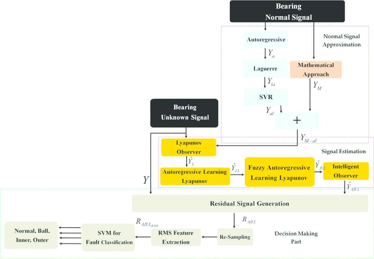
The artificial-based observer, combination of the mathematical-autoregressive learning modeling, and support vector machine for fault detection and identification.
Therefore, first, mathematical modeling of the vibration signal with five degrees of freedom (DOF) is recommended. Additionally, the autoregression technique is used to mathematically model the normal vibration signal. In the next step, the autoregressive technique must be strengthened; this is done using the Laguerre input-output filter. Then, the accuracy of the modeling is increased by SVR. Therefore, by combining autoregressive learning, Laguerre filter, and SVR, the bearing vibration signal is modeled in the NRM. In the second step shown in Figure 1, the main goal is to design a robust, stable, and flexible estimator. Therefore, first, the Lyapunov estimator is suggested.
To overcome the nonlinear part of the vibration signal, the autoregressive learning technique from the modeling part is added to this part and strengthens the signal estimation property. The combination of TSK fuzzy algorithm with the Lyapunov autoregressive learning technique is used to reduce the challenge of uncertainties.
Finally, an adaptive procedure is combined with the fuzzy Lyapunov autoregressive learning technique to increase the flexibility and the quality of the estimation. As shown in Figure 1, fault detection and identification occur in the last step. In this step, first, the residual signal is calculated as the difference between the original and estimated signals. Next, the amount of the signal’s root means square (RMS) is determined; finally, the RMS of the residual signal is identified by classification algorithms such as SVM. This article has the following contributions:
The combination of mathematical-based vibration signal modeling and autoregressive learning techniques is used for vibration signal approximation of a bearing.
The adaptive fuzzy autoregressive learning Lyapunov scheme is suggested for signal estimation in different conditions.
The combination of mathematical-based vibration signal modeling and autoregressive learning techniques for vibration signal approximation, the adaptive fuzzy autoregressive learning Lyapunov scheme for signal estimation, and SVM for classification of bearing fault in one frame.
The structure of this article is as follows: The Case Western Reverse University (CWRU) bearing dataset is described in the second section. In the third section, the vibration signals for the NRM are modeled using the combination of mathematical-based vibration signal modeling and autoregressive learning techniques. The proposed adaptive fuzzy autoregressive learning Lyapunov algorithm for signal estimation, the vibration residual signal generation, determination of the RMS of residual signals, and classification using SVM for fault detection and identification are explained in the fourth section. The results are discussed in Section 5. Finally, the conclusions are provided in Section 6.
2. DATASET
The CWRU dataset is selected to test the proposed scheme and compare it with two state-of-the-art algorithms. In the CWRU dataset, a 2-horsepower (hp) induction motor is utilized to rotate the bearing at various speeds. A vibration sensor collects normal and abnormal vibration signals with a sampling rate of 48 kHz. The bearing used in the CWRU dataset is the 6205-2RS JEM SKF roller bearing; its parameters are given in Table 1. In this dataset, four different classes are defined: NRM, ball fault (BLF), inner race fault (IRF), and outer race fault (ORF). The vibration signal in the NRM is modeled and estimated at 0-hp. Then, the normal signal and abnormal signals with 0.007-inch, 0.014-inch, and 0.021-inch crack sizes are recorded for 0-hp, 1-hp, 2-hp, and 3-hp torque loads. Figure 2 shows the CWRU test bench for data collection. Table 2 shows the data description for the CWRU dataset in normal and abnormal states [31].
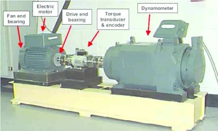
Case Western Reverse University (CWRU) data collection center [28].
| Parameters | Value |
|---|---|
| Number of balls | |
| Stiffness of ball | |
| Mass of outer (kg) | |
| Stiffness of outer | |
| Mass of shaft (kg) | |
| Stiffness of shaft | |
| Damping | |
| Ball diameter | |
| Pitch diameter | |
| Defect size | |
| Defect depth |
Parameters of Case Western Reverse University (CWRU) bearing for mathematical modeling [29].
| Dataset Group | C | Load (hp) | Crack Sizes (in) |
|---|---|---|---|
| i | NRM | 0 | 0.007, 0.014, and 0.021 |
| BLF | 0 | ||
| IRF | 0 | ||
| ORF | 0 | ||
| ii | NRM | 1 | 0.007, 0.014, and 0.021 |
| BLF | 1 | ||
| IRF | 1 | ||
| ORF | 1 | ||
| iii | NRM | 2 | 0.007, 0.014, and 0.021 |
| BLF | 2 | ||
| IRF | 2 | ||
| ORF | 2 | ||
| iv | NRM | 3 | 0.007, 0.014, and 0.021 |
| BLF | 3 | ||
| IRF | 3 | ||
| ORF | 3 |
NRM, normal condition; BLF, ball fault; IRF, inner race fault; ORF, outer race fault.
3. SIGNAL MODELING
In this section, the vibration signal of the bearing in the NRM is modeled using five DOF mathematical modeling of the vibration signal and autoregressive learning algorithm. The mathematical technique (MAT) is a reliable algorithm for modeling the bearing, but it has limitations in an uncertain state. The combination of autoregressive and machine learning techniques is prescribed to increase the accuracy under uncertain conditions [28,29].
3.1. Mathematical Modeling of Bearing
The mathematical modeling of a 5-DOF vibration signal under NRMs in the bearing is expressed by the following equation:
Here,
Here,
Here,
Here,
The ball angular position is defined as
Here,
Therefore, the state-space mathematical modeling of the bearing is represented as the following equation:
Here,
3.2. Autoregressive Learning Algorithm for Bearing Signal Approximation
The core of this work is the design of an artificial intelligence-based observer to identify bearing faults using an estimation algorithm. Thus, the first step is to extract the state-space equation from the bearing vibration signal. Therefore, the autoregressive technique in combination with Laguerre bearing signal filter and support vector regression (SVR) that from now on, it will be called autoregressive learning technique is introduced. The first step is modeling the bearing vibration signal using the autoregressive algorithm [24].
Here,
To improve the robustness of the autoregressive technique, the Laguerre algorithm is recommended [30]. The Laguerre-autoregressive filter technique and the error are represented by the following state-space algorithms [28,29].
Here,
Here,
Here,
Then
While
Therefore, the above formulation is rewritten as
Thus, the bias is calculated using the following equation:
Here,
Here,
Here,
Here,
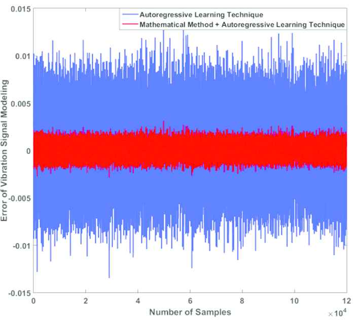
Error of bearing modeling using autoregressive learning technique and the combination of mathematical system modeling and autoregressive learning approach.
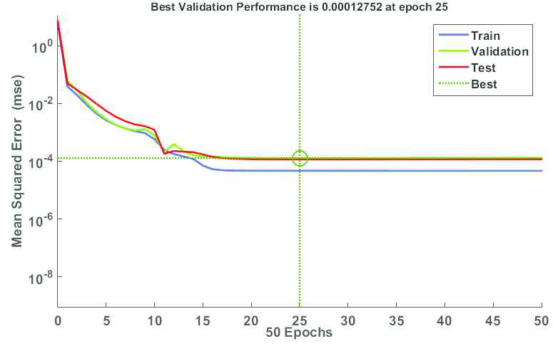
Training, validation, and testing MSE curves during the training of the combination of mathematical system modeling and autoregressive learning approach.
4. ADAPTIVE FUZZY AUTOREGRESSIVE LEARNING LYAPUNOV OBSERVER FOR VIBRATION BEARING SIGNAL ESTIMATION
Based on Figure 1, the vibration signal of the bearing in the NRM was modeled by the combination of 5-DOF mathematical-based vibration signal modeling and autoregressive learning algorithm. Next, the state-space equation of vibration signal in NMR was extracted using Eq. (25). In this section, an artificial intelligence-based observer using a combination of a robust Lyapunov observer, autoregressive learning approach, and adaptive fuzzy technique is designed to estimate the vibration bearing signal. The following steps are used to design the artificial intelligence-based observer: (a) design the robust Lyapunov observer to estimate the normal vibration signal of bearing, (b) solve the challenge of the nonlinear part of signal estimation using the combination of autoregressive learning approach and Lyapunov observer, (c) to improve the flexibility, the combination of fuzzy algorithm, autoregressive learning approach, and Lyapunov observer is recommended, and (d) to increase the stability and reliability the combination of adaptive fuzzy, autoregressive learning approach, and Lyapunov observer is used in this work. Therefore, this section has two main sub-sections: (a) artificial intelligence-based observer based on the combination of Lyapunov observer, autoregressive learning approach, and adaptive fuzzy and (b) fault decision using the combination of residual signal generation and SVM.
4.1. Intelligence-Based Observer
Designing a nonlinear observer, especially with high stability and robustness, is a complicated and difficult task. Various methods have been introduced as observers, but in this section, we will introduce Lyapunov’s technique. The Lyapunov based observer is described by Eq. [34]:
Here,
Here,
The error of the original vibration estimation signal using the Lyapunov-based observer and the error of the uncertainty estimation using the Lyapunov-based observer are represented by the following mathematical definitions:
Here,
Here,
Here,
The nonlinear term of the Lyapunov-based observer is estimated by the autoregressive learning approach using the following mathematical definition:
Here,
Here,
To address the next issue- improve the flexibility of the autoregressive learning Lyapunov-based observer, the fuzzy technique is recommended. The T-S fuzzy observer is used based on the following definition [35]:
Here,
Here,
Here,
To address the final issue, improving the robustness and reliability of the fuzzy autoregressive learning Lyapunov-based observer, the adaptive procedure is recommended. Based on Eqs. (39) and (40), various coefficients for tuning the observer are defined in this algorithm such as
Here,
Here,
4.2. Fault Detection and Identification
As shown in Figure 1, the normal signal was approximated using a combination of MATs and the autoregressive learning approach. After that, the adaptive fuzzy autoregressive learning Lyapunov-based observer (intelligence-based observer) was designed to improve the power of the estimation technique. In this section, the residual signal is determined, which is the difference between the original and estimated signals. Based on this definition, the residual signal is represented by the following technique:
Here,
After resampling the residual signals of the bearing, statistical features such as the RMS are extracted from the resampled residual signals. The following equation represents the RMS of the residual signals:
Here,
Here,
Here,
Here,
If
After specifying the threshold expanse using the SVM, the fault can be detected and its type can be specified. Algorithm 1 represents the proposed technique, which is a combination of intelligence-based observer and SVM for fault detection and identification of bearing systems.
Algorithm 1 Intelligence-based observer and SVM for fault detection and identification in the bearing.
Step 1: Signal Modeling
1: Approximate the bearing function from the vibration signals using MATs. (10)
Detail
1.1 Solve
1.2 Solve
1.3 Solve
1.4
1.5 Compute
1.6 Compute
2: Approximate the bearing function from normal vibration signal using autoregressive technique. (11)
Detail
2.1 Calculate
2.2 Compute
2.3 Compute
3: Improve the robustness of Eq. (11) using autoregressive algorithm with the Laguerre filter. (13)
Detail
3.1 Calculate
3.2 Calculate
3.3 Calculate
4: Increase the accuracy and nonlinearity of Eq. (13) using the autoregressive learning approach. (23)
Detail
4.1 Compute
4.2 Calculate
4.3 Compute
4.4 Calculate
4.5 Compute
4.6 Calculate
4.7 Compute
Step 2: Signal Estimation
5: Signal estimation using robust Lyapunov-based observer. (26–28)
Detail
5.1 Compute
5.2 Calculate
5.3 Compute
5.4 Calculate
6: Estimate the nonlinearity of robust Lyapunov-based observer using autoregressive learning Lyapunov-based observer. (34,35)
Detail
6.1 Compute
6.2 Calculate
6.3 Solve
6.4 Compute
7: Increase the accuracy and flexibility using the fuzzy autoregressive learning Lyapunov-based observer. (39,40)
Detail
7.1 Calculate
7.2 Solve
7.3 Compute
7.4 Calculate
8: Increase the stability, accuracy, and robustness using an adaptive fuzzy autoregressive learning Lyapunov-based observer. (43,44)
Detail
8.1 Solve
8.2 Compute
8.3 Calculate
8.4 Solve
Step 3: Decision Making
9: Generate the residual signal. (46)
10: Resample and extract the RMS feature from residual signal. (47)
11: Fault detection and classification using SVM. (48)
Detail
11.1 Compute
11.2 Calculate
11.3 Find
11.4 Compute
5. RESULTS
To test the power of fault detection and identification, the CWRU dataset is used in this work. This vibration dataset has four classes: NRM, BLF, IRF, and ORF. Table 3 shows the window characterizations for estimated and verification signals from the CWRU bearing vibration dataset. Figure 5 illustrates these classes when the torque load and crack size are 0-hp and 0.007-inch, respectively.
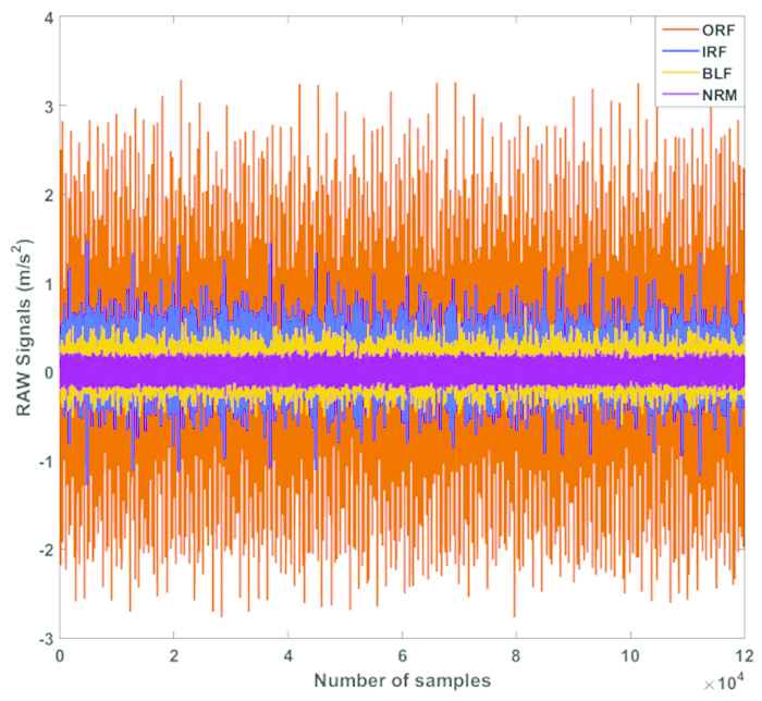
Different classes from Case Western Reverse University (CWRU) dataset for 0-hp and 0.007-inch crack.
| Classes | Number of Samples |
|---|---|
| Samples per state | 100 |
| Samples per classes | 4*100 = 400 |
| Training samples per state | 60 |
| Training samples per classes | 240 |
| Validating samples per state | 15 |
| Validating samples per classes | 60 |
| Testing samples per state | 25 |
| Testing samples per state | 100 |
Case Western Reverse University (CWRU) window characterization for training and testing: CWRU data.
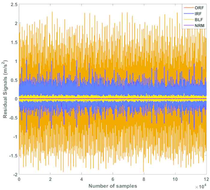
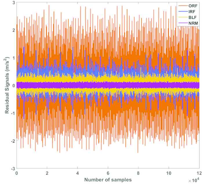
To test the effectiveness of the bearing fault classification using the intelligence-based observer + SVM, this method is validated and compared with two state-of-the-art techniques: the autoregressive learning Lyapunov-based approach + SVM and the Lyapunov-based technique + SVM. Figures 6–8 illustrate the residual signals for the four classes using the intelligence-based observer, autoregressive learning Lyapunov-based approach, and Lyapunov-based technique, respectively.
Residual signals using proposed intelligence-based observer.

Residual signals using autoregressive learning Lyapunov-based approach.
Residual signals using Lyapunov-based technique.
Based on these figures, it can be seen that the intelligence-based observer has better separability than the autoregressive learning Lyapunov-based approach and Lyapunov-based technique. Based on Figures 6 and 7, the detectability in the autoregressive learning Lyapunov-based approach is better than that of the Lyapunov-based technique. Figure 9 compares the RMS values of the residual signals calculated by the intelligence-based observer, autoregressive learning Lyapunov-based approach, and Lyapunov-based technique. According to this figure, fault detection accuracy, which is the discrimination of normal from abnormal signals, is exceptional in all three algorithms.
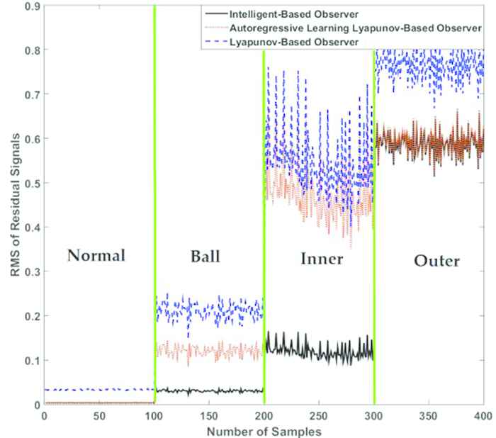
Root mean square (RMS) of residual signals using proposed intelligence-based observer, autoregressive learning Lyapunov-based approach, and Lyapunov-based technique.
As shown in these figures, the classification accuracy for the proposed algorithm (intelligence-based observer) is better than those of the other two methods. The main problem of fault identification in the autoregressive learning Lyapunov-based approach and Lyapunov-based technique is related to anomaly identification for inner and outer defects.
The K-fold cross-validation is used to validate the accuracy and precision of the intelligent-based observer + SVM (proposed scheme), autoregressive learning Lyapunov-based observer + SVM, and Lyapunov-based observer + SVM, respectively. To produce the stable results, the K in the experiment is 5 and the average of accuracy shows in Tables 4–6 and Figures 10–12.

Confusion matrix to calculate the average fault diagnosis accuracy and precision using intelligent-based observer + support vector machine (SVM) for various crack sizes (0.007-inch, 0.014-inch, and 0.021-inch) and different torque loads (0-hp, 1-hp, 2-hp, and 3-hp).
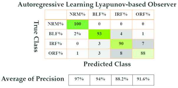
Confusion matrix to calculate the average fault diagnosis accuracy and precision using autoregressive learning Lyapunov-based observer + support vector machine (SVM) for various crack sizes (0.007-inch, 0.014-inch, and 0.021-inch) and different torque loads (0-hp, 1-hp, 2-hp, and 3-hp).
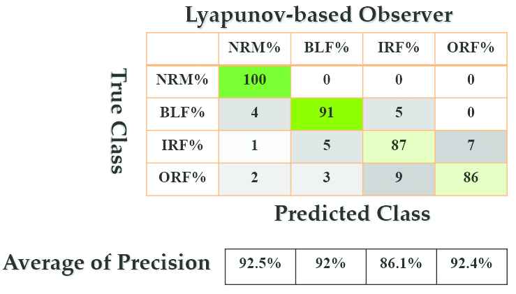
Confusion matrix to calculate the average fault diagnosis accuracy and precision using Lyapunov-based observer + support vector machine (SVM) for various crack sizes (0.007-inch, 0.014-inch, and 0.021-inch) and different torque loads (0-hp, 1-hp, 2-hp, and 3-hp).
| Algorithm | Intelligence-Based Observer + SVM | |||
|---|---|---|---|---|
| Torque Load | 0-hp (%) | 1-hp (%) | 2-hp (%) | 3-hp (%) |
| NRM | 100 | 100 | 100 | 100 |
| BLF | 97.3 | 97.3 | 91.3 | 93.3 |
| IRF | 94.7 | 93.3 | 98.7 | 94.7 |
| ORF | 98.3 | 96 | 100 | 98.3 |
| Average | 97.6 | 96.7 | 97.5 | 96.6 |
SVM, support vector machine; NRM, normal condition; BLF, ball fault; IRF, inner race fault; ORF, outer race fault.
The average fault diagnosis accuracy using intelligence-based observer + SVM for crack sizes of 0.007-inch, 0.014-inch, and 0.021-inch.
| Algorithm | Autoregressive learning Lyapunovbased observer + SVM | |||
|---|---|---|---|---|
| Torque Load | 0-hp (%) | 1-hp (%) | 2-hp (%) | 3-hp (%) |
| NRM | 100 | 100 | 100 | 100 |
| BLF | 93 | 91 | 97.3 | 90.7 |
| IRF | 88 | 92 | 92 | 88 |
| ORF | 90.3 | 84.3 | 89.7 | 88 |
| Average | 92.8 | 91.8 | 94.8 | 91.7 |
SVM, support vector machine; NRM, normal condition; BLF, ball fault; IRF, inner race fault; ORF, outer race fault.
The average fault diagnosis accuracy using autoregressive learning Lyapunov-based approach + SVM for crack sizes of 0.007-inch, 0.014-inch, and 0.021-inch.
| Algorithm | Lyapunov-Based Observer + SVM | |||
|---|---|---|---|---|
| Torque Load | 0-hp (%) | 1-hp (%) | 2-hp (%) | 3-hp (%) |
| NRM | 100 | 100 | 100 | 100 |
| BLF | 89.7 | 93.3 | 92.7 | 88.3 |
| IRF | 82 | 88 | 88 | 90 |
| ORF | 87 | 83 | 86 | 88 |
| Average | 89.7 | 91 | 91.7 | 91.6 |
SVM, support vector machine; NRM, normal condition; BLF, ball fault; IRF, inner race fault; ORF, outer race fault.
The average fault diagnosis accuracy using Lyapunov-based observer + SVM for crack sizes of 0.007-inch, 0.014-inch, and 0.021-inch.
Tables 4–6 illustrate the power of fault identification using the intelligence-based observer, autoregressive learning Lyapunov-based approach, and Lyapunov-based technique when the torque load varies between 0-hp and 3-hp.
Based on the above tables, the fault identification accuracy of the proposed scheme is much better than those of the other two methods. In addition, the average accuracy of the intelligence-based observer + SVM is about 97.1%, whereas in the autoregressive learning Lyapunov-based approach + SVM and Lyapunov-based technique + SVM it is 92.8% and 91%, respectively. Thus, the proposed algorithm improved the average fault identification accuracy by 4.3% and 6.1% compared to the autoregressive learning Lyapunov-based approach + SVM and Lyapunov-based technique + SVM, respectively. Figures 10–12 show the confusion matrices of these algorithms. Based on these figures, these confusion matrices are the average accuracy and precision for various crack sizes and different torque loads. Regarding these figures, it is clear that the average accuracy and precision for the proposed scheme is better than the other methods. The range of misclassification in the proposed method is less than the others.
6. CONCLUSION
The principal purpose of this work was to solve the challenge of identification and classification of faults in a bearing. The combination of mathematical and autoregressive learning approaches, an intelligence-based observer, and the SVM were considered to address this issue. This approach consists of four main steps. First, the signal was modeled in normal operation using a combination of mathematical vibration signal modeling and autoregressive learning vibration signal approximation techniques. After modeling the normal vibration signal, the signal was estimated using a combination of the modern control algorithm and machine learning techniques. To approximate the signal, first, the robust Lyapunov-based technique was selected, and in later stages, this procedure was modified. Next, the problem of nonlinear parameters was solved by combining the Lyapunov-based observer method with an autoregressive learning scheme. To increase the flexibility, the autoregressive learning Lyapunov-based observation technique was combined with a fuzzy logic approach. Finally, to improve the accuracy and increase the robustness, the fuzzy autoregressive learning Lyapunov-based observer was combined with the adaptive technique. In the final step, the fault was classified and identified by the SVM. The proposed algorithm improved the average fault identification accuracy by 3.9% and 5.2% compared to the autoregressive learning Lyapunov-based approach and Lyapunov-based observer, respectively.
CONFLICTS OF INTEREST
The authors declare no conflict of interest.
AUTHORS' CONTRIBUTIONS
All of the authors contributed equally to the conception of the idea, the design of experiments, the analysis and interpretation of results, and the writing of the manuscript. Writing—original draft preparation, F.P. and J.-M.K.; writing—review and editing, F.P. and J.-M.K. All authors have read and agreed to the published version of the manuscript.
FUNDING STATEMENT
This work was supported by the Korea Institute of Energy Technology Evaluation and Planning (KETEP) and the Ministry of Trade, Industry & Energy (MOTIE) of the Republic of Korea (No. 20192510102510).
ACKNOWLEDGMENTS
This work was supported by the Korea Institute of Energy Technology Evaluation and Planning (KETEP) and the Ministry of Trade, Industry & Energy (MOTIE) of the Republic of Korea (No. 20192510102510).
REFERENCES
Cite this article
TY  - JOUR
AU  - Farzin Piltan
AU  - Jong-Myon Kim
PY  - 2021
DA  - 2021/01/04
TI  - Fault Diagnosis of Bearings Using an Intelligence-Based Autoregressive Learning Lyapunov Algorithm
JO  - International Journal of Computational Intelligence Systems
SP  - 537
EP  - 549
VL  - 14
IS  - 1
SN  - 1875-6883
UR  - https://doi.org/10.2991/ijcis.d.201228.002
DO  - 10.2991/ijcis.d.201228.002
ID  - Piltan2021
ER  -