International Journal of Computational Intelligence Systems

Volume 14, Issue 1, 2021, Pages 503 - 527

Algorithm for Multiple Attribute Decision-Making with Interactive Archimedean Norm Operations Under Pythagorean Fuzzy Uncertainty

Authors
Lei Wang1, *, ORCID, Harish Garg2, *, ORCID
1Department of Basic Teaching, Liaoning Technical University, Huludao, 125105, China
2School of Mathematics, Thapar Institute of Engineering and Technology, Deemed University, Patiala 147004, India
*Corresponding author. Email: lntuwl@126.com and harishg58iitr@gmail.com
Corresponding Authors
Lei Wang, Harish Garg
Received 11 September 2020, Accepted 2 December 2020, Available Online 24 December 2020.
DOI
10.2991/ijcis.d.201215.002How to use a DOI?
Keywords
Multiple attribute decision-making; Archimedean norm; Pythagorean fuzzy sets; Aggregation operators; Operation laws
Abstract

Recently, a great attention is paid toward developing aggregation operators for Pythagorean fuzzy set (PFS). However, few of them have adopted the rules of Archimedean t-conorm and t-norm (ATT) to aggregate the numbers. Motivated by this, the keep interest of the present work is to define some Pythagorean fuzzy interaction aggregation operators with the aid of ATT. To do this, the objective of the work is divided into three folds. In the first fold, we define some interactive operations law for PFSs and propose their corresponding new interaction Pythagorean operators, namely Archimedean based Pythagorean fuzzy interactive weighted averaging (A-PFIWA) operator and Archimedean based Pythagorean fuzzy interactive weighted geometric (A-PFIWG) operator. In the second fold, we investigate their desirable properties and study the several special cases of the proposed ones with respect the existing ones. Lastly, we design an algorithm to solve the multiple attribute decision-making issues with Pythagorean fuzzy uncertainties and explain their utilization with a numerical example. Further, several examples are discussed to demonstrate the validity and superiority of the proposed method. The novelties of proposed operators are that they not only can offer a more flexible method via selecting diverse forms of ATT, but also can reflect the interactive influence among membership degree and nonmembership degree for PFSs.

Copyright
© 2021 The Authors. Published by Atlantis Press B.V.
Open Access
This is an open access article distributed under the CC BY-NC 4.0 license (http://creativecommons.org/licenses/by-nc/4.0/).

1. INTRODUCTION

Multiple attribute decision-making (MADM) issue involving a series of approaches to choose optimal alternative or acquire their priority ordering in accordance with given attribute [1], which is a major branch of modern decision science. Considering the complicacy of the realistic decision circumstances, decision makers (DMs) may realize that it is difficult to describe crisp values about attribute evaluation information. For this, the theory of intuitionistic fuzzy set (IFS) [2] was initiated by Atanassov in 1986, it suits for tackling the issue of insufficient evaluation information. IFS expresses attribute evaluation information by membership degree (MD), nonmembership degree (NMD) and hesitation degree, respectively, which is a useful extension of fuzzy sets [3]. Nowadays, plenty of researches [48] have been implemented on MADM techniques within intuitionistic fuzzy information.

More recently, the notion of Pythagorean fuzzy sets (PFS) was explored by Yager [9,10] as a useful assessment technique, which is successful extension of IFS. Similar to IFS, PFS is also represented by MD and NMD, the sum of MD and NMD are permitted to bigger than one, but the square sum of these two degrees is not exceed than one. Therefore, PFS possesses more superiority comparing with IFS to express the indeterminacy in both theory and application aspects [1115]. In the field of MADM, some classical evaluation approaches are extend to PFS, including LINAMP [16], TODIM [17], VIKOR [18], ELECTRE [19] and so on. Zhang and Xu [20] developed detailed mathematical structure representation for PFS, they also proposed the notion of Pythagorean fuzzy numbers (PFNs), and corresponding fundamental operations on PFNs. Meanwhile, they developed ranking rules over PFNs by defined scores function. Additionally, they explored the distance between PFNs, and combined it and TOPSIS method to address Pythagorean fuzzy MADM issues. Apart from above mentioned evaluation methods, a large number of aggregation operators (AOs) [2130] were proposed by some scholars to fuse PFNs employing the operations provided by Ref. [20]. For instance, in the light of the ordered weighted averaging (OWA) operator [31], Zhang [21] defined the Pythagorean fuzzy OWA operator and utilized it to manage group decision-making issue. Enlightened by the work [5], Ma and Xu [22] defined the Pythagorean fuzzy weighted averaging (PFWA) operator. Further, considering the information about MD and NMD should be equally handled, they initiated neutrality AOs, that is, symmetric PFWA, and also discussed the relationships over these AOs. Zeng et al. [23] discussed the Pythagorean fuzzy induced OWA weighted average operator and corresponding decision approach for settling group decision problems in Pythagorean fuzzy setting. In Ref. [24], several generalized Pythagorean fuzzy averaging AOs were presented utlizing the Einstein t-norm and t-conorm. Garg [25] proposed neutrality Pythagorean fuzzy geometric AOs for aggregating PFNs. Yang et al. [26] developed a series of Frank power AOs for interval-valued PFNs. Wu and Wei [27] created several Hamacher AOs to settle MADM issues with Pythagorean fuzzy information. Besides, in view of the relationship of attributes, some AOs [2830] are initiated. However, Wei [32] pointed that the ranking orders are not reasonable by using above AOs [2130] in some situations. For instance, let β1=(μ1,ν1) and β2=(μ2,ν2) be two PFNs, when μ1=0 and μ20, then employing the multiplication operation in [20], we obtain μβ1β2=0. Which indicates that regardless of the value of MD μ2, the outcome μβ1β2=0 can be obtained always, it's an unreasonable situation. Similarly, the outcome νβ1β2=0 is always kept based on the addition operation in [20], when ν1=0 and ν20. It's also an irrational situation. In order to overcome these shortcomings, enlightened by the idea [33] he defined the interactive operations on PFNs, and proposed various Pythagorean fuzzy AOs with the help of interactive operations, including Pythagorean fuzzy interactive weighted average, weighted geometric, ordered weighted average, ordered weighted geometric, hybrid average and hybrid geometric, labeled by PFIWA, PFIWG, PFIOWA, PFIOWG, PFIHA and PFIHG, respectively. After the work [33], certain interactive AOs [3436] were presented within intuitionistic fuzzy circumstances. Based on the interactive operations [32], Gao et al. [37] proposed several interactive power AOs, which can reduce the impact of confused data on integration results. Taking the relationship over aggregated information into account, Wang and Li [38] explored the Pythagorean fuzzy interactive power Bonferroni means (BM) operator and weight form along with their properties and special cases. Zhu et al. [39] built interactive power partitioned BM operators for PFNs. Li et al. [40] created several new Pythagorean fuzzy interactive hybrid weighted AOs, the merit of these AOs is that possess the property of idempotency.

Meanwhile, alternative and appropriate operational laws play a crucial role in AOs. The Archimedean t-conorm and t-norm (ATT) [41,42] are formed using an additive function and a dual function. When the additive function was chosen with different expressions, ATT reduced to various t-conorm and t-norm, they are the Algebraic, Einstein, Hamacher and Frank t-conorms and t-norms and so on. ATT has been extended to diverse fuzzy circumstances, including IFSs [43,44], interval-valued hesitant fuzzy set [45], single-valued neutrosophic set [46] and dual hesitant fuzzy set [47]. Recently, based on the ATT, Yang et al. [48] proposed two Pythagorean fuzzy BM AOs for PFNs, and applied them to match investment selection problem.

From the above discussions, the existing operators [32], [27] for Pythagorean fuzzy information have the following two limitations:

  1. Although the AOs presented in [32,37,38] can capture the interactions between MD and NMD for Pythagorean fuzzy information, the operational laws of these AOs only adopted algebra t-conorm and t-norm. It cannot offer a more flexible result.

  2. AOs provided in [24,25,27] employing the Einstein and Hamacher operations, respectively, but they cannot acquire reasonable decision-making outcomes under some cases.

Clearly, the ATT [41,48] is a good alternative to avoid the first limitation, which contains many different types of the t-conorm and t-norm, and the algebra form is the special case of ATT. Interactive operations [32] can overcome the second limitation effectively via capturing the interactions between MD and NMD.

On the basis of above analysis, the main intentions of this study are:

  1. To explore several novel interactive averaging and geometric AOs about PFNs to avoid the above two limitations with the aid of ATT.

  2. To obtain some important properties and some specific cases of the defined newly AOs.

  3. To build a new MADM approach by using the proposed interactive AOs in Pythagorean fuzzy context.

  4. To demonstrate the availability and the merits of the constructed MADM approach.

An outline of this research is listed as follows: Section 2 concisely recalls the fundamental knowledge of PFSs, interactive operations on PFSs, and ATT. In Section 3, we define certain interactive operational rules on PFSs with the help of ATT. In Section 4, we propose Archimedean based PFIWA (A-PFIWA) and Archimedean based PFIWG (A-PFIWG) operators, and we discuss their desirable properties. In Section 5, we build a novel MADM technique utilizing the constructed A-PFIWA and A-PFIWG operators and in Section 6 we utilize a actual instance to show our technique and compare it with the previous research. Finally, Section 7 concludes the paper.

2. PRELIMINARIES

Some preconditions for PFS, interactive operational rules of PFS and ATT are briefly provided in this section.

2.1. Pythagorean Fuzzy Set

Definition 2.1.

[9,10] A PFS P on universal set Z is defined as:

P=z,μP(z),νP(z)zZ.(1)
where μP(z),νP(z) stand for the MD and NMD for each zZ, respectively, which meets the conditions: μP(z),νP(z)[0,1]and μP(z)2+νP(z)2[0,1]. Indeterminacy degree is πP(z)=1μP(z)2νP(z)2.

Zhang and Xu [20] defined β=(μβ,νβ) as a PFN with μβ,νβ[0,1] and μβ2+νβ2[0,1]. All PFNs are denoted by Ω. Wei [32] defined interactive operational laws for PFNs.

Definition 2.2.

Suppose β=(μβ,νβ),β1=(μβ1,νβ1)and β2=(μβ2,νβ2) are three PFNs, then the interactive operations are provided in the following expressions [32]:

(1)β1β2=μβ12+μβ22μβ12μβ22,νβ12+νβ22νβ12νβ22μβ12νβ22νβ12μβ22;(2)β1β2=μβ12+μβ22μβ12μβ22μβ12νβ22νβ12μβ22,νβ12+νβ22νβ12νβ22;(3)kβ=1(1μβ2)k,(1μβ2)k(1(μβ2+νβ2))k,k>0;(4)βk=(1νβ2)k(1(μβ2+νβ2))k,1(1νβ2)k,k>0.

Zhang and Xu [20] also have given the comparison rules for two PFNs.

Definition 2.3.

[20] Let β=(μβ,νβ) be a PFN, the score and accuracy of β are expressed by s(β)=μβ2νβ2 and a(β)=μβ2+νβ2, respectively. Suppose β1,β2 are two PFNs, the following two expressions, as long as one holds

  1. s(β1)>s(β2);

  2. s(β1)=s(β2) and a(β1)>a(β2).

then β1β2.

2.2. Archimedean t-conorm and t-norm

The notions of Archimedean t-norm and t-conorm were initiated by Klir and Yuan [41] and Nguyen and Walker [42], the formal definitions shown as follows:

Definition 2.4.

[41,42] A t-norm is a mapping T:[0,1]2[0,1], and meets the following properties:

  1. T(1,a)=a, for all a;

  2. T(a,b)=T(b,a), for all a and b;

  3. T(a,T(b,c))=T(T(a,b),c), for all a, b and c;

  4. If ab and cd then T(a,c)T(b,d).

Definition 2.5.

[41,42] A t-conorm is a mapping T:[0,1]2[0,1], and meets the following properties:

  1. T(0,a)=a, for all a;

  2. T(a,b)=T(b,a), for all a and b;

  3. T(a,T(b,c))=T(T(a,b),c), for all a, b and c;

  4. If ab and cd then T(a,c)T(b,d).

Ref. [49] indicated that a strict Archimedean t-norm is depicted through its following additive continuous function l:

T(a,b)=l1(l(a)+l(b))(2)

In which l:[0,1][0,+) is a strictly decreasing function and l(1)=0.

Analogously, utilized to its dual t-conorm, the following expression can be derived:

T(a,b)=h1(h(a)+h(b))(3)
where h(r)=l(1r).

3. ATT ON PFNs

Enlightened by the idea [50] and Equations (2) and (3), next, we shall develop new interactive operations rules for PFNs in the light of ATT.

Definition 3.1.

Suppose β=(μβ,νβ),β1=(μβ1,νβ1) and β2=(μβ2,νβ2) are three PFNs, then the novel operational rules for PFNs applying ATT are defined as follows:

β1β2=T(μβ12,μβ22),T(μβ12+νβ12,μβ22+νβ22)T(μβ12,μβ22)(4)
β1β2=T(μβ12+νβ12,μβ22+νβ22)T(νβ12,νβ22),T(νβ12,νβ22)(5)

Further, we can deduce

β1β2=h1(h(μβ12)+h(μβ22)),h1(h(μβ12+νβ12)+h(μβ22+νβ22))h1(h(μβ12)+h(μβ22))(6)
β1β2=h1(h(μβ12+νβ12)+h(μβ22+νβ22))h1(h(νβ12)+h(νβ22)),h1(h(νβ12)+h(νβ22))(7)
kβ=h1(kh(μβ2)),h1(kh(μβ2+νβ2))h1(kh(μβ2)),k>0(8)
βk=h1(kh(μβ2+νβ2))h1(kh(νβ2)),h1(kh(νβ2)),k>0(9)

Proof.

Now, we shall verify the Equations (6) and (8) and the others are similar.

With the help of Equation (3), we have

0h1(h(μβ12)+h(μβ22))1,0h1(h(μβ12+νβ12)+h(μβ22+νβ22))1.

Since h() is a strictly increasing function, so we can obtain

h1(h(μβ12+νβ12)+h(μβ22+νβ22))h1(h(μβ12)+h(μβ22)),
which further gives that
0h1(h(μβ12+νβ12)+h(μβ22+νβ22))h1(h(μβ12)+h(μβ22))1.

Moreover,

0h1(h(μβ12)+h(μβ22))2+h1(h(μβ12+νβ12)+h(μβ22+νβ22))h1(h(μβ12)+h(μβ22))2=h1h(μβ12+νβ12)+h(μβ22+νβ22)1.

Hence, Equation (6) holds.

Similarly, from Equation (3), we get

0h1(kh(μβ2))1,0h1(kh(μβ2+νβ2))1.

As h() is a strictly increasing function, then we have h1(kh(μβ2+νβ2))h1(kh(μβ2)), that is 0h1(kh(μβ2+νβ2))h1(kh(μβ2))1. Additionally,

0h1(kh(μβ2))2+h1(kh(μβ2+νβ2))h1(kh(μβ2))2=h1kh(μβ2+νβ2)1.

So, Equation (8) holds.

If we set specific expressions to the function l, then the following several fundamental t-conorms and t-norms can be obtained:

  • Case 1:

    If l(r)=log(r), then h(r)=log(1r), l1(r)=et and h1(r)=1er, based on Definition 3.1, we have

    (1)β1β2=μβ12+μβ22μβ12μβ22,νβ12+νβ22νβ12νβ22μβ12νβ22νβ12μβ22(10)
    (2)β1β2=μβ12+μβ22μβ12μβ22μβ12νβ22νβ12μβ22,νβ12+νβ22νβ12νβ22(11)
    (3)kβ=1(1μβ2)k,(1μβ2)k(1(μβ2+νβ2))k(12)
    (4)βk=(1νβ2)k(1(μβ2+νβ2))k,1(1νβ2)k(13)
    which are Algebraic interactive operations on PFNs defined by Wei [32].

  • Case 2:

    If l(r)=log(2rr), then h(r)=log(1+r1r), and h1(r)=er1er+1, from Definition 3.1, we get

    (1)β1β2=j=12(1+μβj2)j=12(1μβj2)j=12(1+μβj2)+j=12(1μβj2),j=12(1+μβj2+νβj2)j=12(1μβj2νβj2)j=12(1+μβj2+νβj2)+j=12(1μβj2νβj2)j=12(1+μβj2)j=12(1μβj2)j=12(1+μβj2)+j=12(1μβj2)(14)
    (2)β1β2=j=12(1+μβj2+νβj2)j=12(1μβj2νβj2)j=12(1+μβj2+νβj2)+j=12(1μβj2νβj2)j=12(1+νβj2)j=12(1νβj2)j=12(1+νβj2)+j=12(1νβj2),j=12(1+νβj2)j=12(1νβj2)j=12(1+νβj2)+j=12(1νβj2)(15)
    (3)kβ=(1+μβ2)k(1μβ2)k(1+μβ2)k+(1μβ2)k,(1+μβ2+νβ2)k(1μβ2νβ2)k(1+μβ2+νβ2)k+(1μβ2νβ2)k(1+μβ2)k(1μβ2)k(1+μβ2)k+(1μβ2)k(16)
    (4)βk=(1+μβ2+νβ2)k(1μβ2νβ2)k(1+μβ2+νβ2)k+(1μβ2νβ2)k(1+νβ2)k(1νβ2)k(1+νβ2)k+(1νβ2)k,(1+νβ2)k(1νβ2)k(1+νβ2)k+(1νβ2)k(17)
    which are called Einstein interactive operations on PFNs.

  • If l(r)=logρ+(1ρ)rr,ρ>0, then h(r)=logρ+(1ρ)(1r)(1r), and h1(r)=er1er+ρ1, according to Definition 3.1, we get

    (1)β1β2=j=12(ρ+(1ρ)(1μβj2))j=12(1μβj2)j=12(ρ+(1ρ)(1μβj2))+(ρ1)j=12(1μβj2),j=12(ρ+(1ρ)(1μβj2νβj2))j=12(1μβj2νβj2)j=12(ρ+(1ρ)(1μβj2νβj2))+(ρ1)j=12(1μβj2νβj2)j=12(ρ+(1ρ)(1μβj2))j=12(1μβj2)j=12(ρ+(1ρ)(1μβj2))+(ρ1)j=12(1μβj2)(18)
    (2)β1β2=j=12(ρ+(1ρ)(1μβj2νβj2))j=12(1μβj2νβj2)j=12(ρ+(1ρ)(1μβj2νβj2))+(ρ1)j=12(1μβj2νβj2)j=12(ρ+(1ρ)(1νβj2))j=12(1νβj2)j=12(ρ+(1ρ)(1νβj2))+(ρ1)j=12(1νβj2),j=12(ρ+(1ρ)(1νβj2))j=12(1νβj2)j=12(ρ+(1ρ)(1νβj2))+(ρ1)j=12(1νβj2)(19)
    (3)kβ=(ρ+(1ρ)(1μβ2))k(1μβ2)k(ρ+(1ρ)(1μβ2))k+(ρ1)(1μβ2)k,(ρ+(1ρ)(1μβ2νβ2))k(1μβ2νβ2)k(ρ+(1ρ)(1μβ2νβ2))k+(ρ1)(1μβ2νβ2)k(ρ+(1ρ)(1μβ2))k(1μβ2)k(ρ+(1ρ)(1μβ2))k+(ρ1)(1μβ2)k(20)
    (4)βk=(ρ+(1ρ)(1μβ2νβ2))k(1μβ2νβ2)k(ρ+(1ρ)(1μβ2νβ2))k+(ρ1)(1μβ2νβ2)k(ρ+(1ρ)(1νβ2))k(1νβ2)k(ρ+(1ρ)(1νβ2))k+(ρ1)(1νβ2)k,(ρ+(1ρ)(1νβ2))k(1νβ2)k(ρ+(1ρ)(1νβ2))k+(ρ1)(1νβ2)k(21)

  • If l(r)=logε1εr1,ε>1, then h(r)=logε1ε1r1, and h1(r)=1logεε1+erer, on the basis of Definition 3.1, we obtain:

    (1)β1β2=1logε1+1ε1j=12(ε1μβj21),logε1+1ε1j=12(ε1μβj21)1+1ε1j=12(ε1μβj2νβj21)(22)
    (2)β1β2=logε1+1ε1j=12(ε1νβj21)1+1ε1j=12(ε1μβj2νβj21),1logε1+1ε1j=12(ε1νβj21)(23)
    (3)λβ=1logε1+(ε1μβ21)λ(ε1)λ1,logε(ε1)λ1+(ε1μβ21)λ(ε1)λ1+(ε1μβ2νβ21)λ(24)
    (4)βλ=logε(ε1)λ1+(ε1νβ21)λ(ε1)λ1+(ε1μβ2νβ21)λ,1logε1+(ε1νβ21)λ(ε1)λ1(25)
    which are called Frank interactive operations on PFNs.

Furthermore, we can verify some operational laws straightforward as follows.

Theorem 3.1.

Suppose β=(μβ,νβ),β1=(μβ1,νβ1) and β2=(μβ2,νβ2) are three PFNs, and real numbers k>0,k1>0,k2>0, then

  1. β1β2=β2β1.

  2. β1β2=β2β1.

  3. k(β1β2)=kβ1kβ2.

  4. (β1β2)k=(β1)k(β2)k.

  5. k1βk2β=(k1+k2)β.

  6. βk1βk2=β(k1+k2).

  7. (βk1)k2=βk1k2.

Proof.

We shall prove the parts (3) and (4), while others parts (1), (2), (5), (6), (7) can be proved analogously.

  1. For PFNs β1=(μβ1,νβ1)and β2=(μβ2,νβ2) and a real k>0, we have

    k(β1β2)=kh1(h(μβ12)+h(μβ22)),h1(h(μβ12+νβ12)+h(μβ22+νβ22))h1(h(μβ12)+h(μβ22))=h1(kh(h1(h(μβ12)+h(μβ22)))),h1(kh(h1(h(μβ12+νβ12)+h(μβ22+νβ22))))h1(kh(h1(h(μβ12)+h(μβ22))))=h1(kh(μβ12)+kh(μβ22)),h1(kh(μβ12+νβ12)+kh(μβ22+νβ22))h1(kh(μβ12)+kh(μβ22))=kβ1kβ2

  2. For PFNs β1 and β2, we have

    (β1β2)k=h1h(μβ12+νβ12)+h(μβ22+νβ22)h1(h(νβ12)+h(νβ22)),h1(h(νβ12)+h(νβ22)))k=h1kh(h1(h(μβ12+νβ12)+h(μβ22+νβ22)))h1(kh(h1(h(νβ12)+h(νβ22)))),h1(kh(h1(h(νβ12)+h(νβ22))))=h1(kh(μβ12+νβ12)+kh(μβ22+νβ22))h1(kh(νβ12)+kh(νβ22)),h1(kh(νβ12)+kh(νβ22))=(β1)k(β2)k

4. ARCHIMEDEAN BASED PYTHAGOREAN FUZZY INTERACTIVE AOs

The focus of this part is to establish some novel interactive AOs for PFNs based on the ATT.

4.1. Archimedean Based Pythagorean Fuzzy Interactive Averaging Operators

Definition 4.1.

Suppose βj=(μβj,νβj)(j=1,2,3,,n) is a group of PFNs, an A-PFIWA operator is a mapping APFIWA:ΩnΩ, meeting

APFIWA(β1,β2,,βn)=j=1nωjβj(26)
where, ω=(ω1,ω2,,ωn)Tis the weight vector of βj(j=1,2,3,,n), satisfing ωj[0,1], j=1nωj=1.

Theorem 4.1.

Suppose βj=(μβj,νβj)(j=1,2,3,,n) is a group of PFNs, then the aggregated outcome employing A-PFIWA operator is also a PFN, and

APFIWA(β1,β2,,βn)=j=1nωjβj=h1j=1nωjh(μβj2),h1j=1nωjh(μβj2+νβj2)h1j=1nωjh(μβj2)(27)

Proof of Theorem 4.1.

We verify Equation (27) via utilizing mathematical induction on n.

  1. When n=2, and by the operations of the PFNs on β1 and β2, we have

    ω1β1=h1(ω1h(μβ12)),h1(ω1h(μβ12+νβ12))h1(ω1h(μβ12))
    ω2β2=h1(ω2h(μβ22)),h1(ω2h(μβ22+νβ22))h1(ω2h(μβ22))
    then
    ω1β1ω2β2=h1h(h1(ω1h(μβ12)))+h(h1(ω2h(μβ22))),h1h(h1(ω1h(μβ12+νβ12)))+h(h1(ω2h(μβ22+νβ22)))h1h(h1(ω1h(μβ12)))+h(h1(ω2h(μβ22)))=h1ω1h(μβ12)+ω2h(μβ22),h1ω1h(μβ12+νβ12)+ω2h(μβ22+νβ22)h1ω1h(μβ12)+ω2h(μβ22)=h1j=12ωjh(μβj2),h1j=12ωjh(μβ12+νβj2)h1j=12ωjh(μβ12)

  2. Assume Equation (27) is true for n=k, that is,

    APFIWA(β1,β2,,βk)=j=1kωjβj=h1j=1kωjh(μβj2),h1j=1kωjh(μβj2+νβj2)h1j=1kωjh(μβj2)

    Then when n=k+1, by Definition 3.1, we obtain

    APFIWA(β1,β2,,βk,βk+1)=APFIWA(β1,β2,,βk)ωk+1βk+1=h1j=1kωjh(μβj2),h1j=1kωjh(μβj2+νβj2)h1j=1kωjh(μβj2)h1(ωk+1h(μβk+12)),h1(ωk+1h(μβk+12+νβk+12))h1(ωk+1h(μβk+12))=h1hh1j=1kωjh(μβj2)+h(h1(ωk+1h(μβk+12))),h1hh1j=1kωjh(μβj2+νβj2)+h(h1(ωk+1h(μβk+12+νβk+12)))h1hh1j=1kωjh(μβ12)+h(h1(ωk+1h(μβk+12)))=h1j=1kωjh(μβj2)+ωk+1h(μβk+12),h1j=1kωjh(μβj2+νβj2)+ωk+1hμβk+12+νβk+12h1j=1kωjh(μβj2)+ωk+1h(μβk+12)=h1j=1k+1ωjh(μβj2),h1j=1k+1ωjh(μβj2+νβj2)h1j=1k+1ωjh(μβj2)

    That is, Equation (27) is true for n=k+1.

    Hence, according to the result of (1) and (2), Equation (27) is true for all n.

    Furthermore, function h(r) is strictly increasing, then

    0h1j=1nωjh(μβj2)2+h1j=1nωjh(μβj2+νβj2)h1j=1nωjh(μβj2)2=h1j=1nωjh(μβj2+νβj2)h1j=1nωjh(1)=h1h(1)j=1nωj=1

    Therefore, the proof is completed.

When we adopt diverse forms of the function l(r), then some especial AOs can be determined as follows:

  • Case 1:

    If l(r)=log(r), according to Theorem 4.1, then A-PFIWA operator becomes the PFIWA operator introduced by Wei [32].

    PFIWA(β1,β2,,βn)=1j=1n(1μβj2)ωj,j=1n(1μβj2)ωjj=1n(1μβj2νβj2)ωj(28)

  • Case 2:

    If l(r)=log(2rr), from Theorem 4.1, A-PFIWA operator becomes

    EPFIWA(β1,β2,,βn)=j=1n(1+μβj2)ωjj=1n(1μβj2)ωjj=1n(1+μβj2)ωj+j=1n(1μβj2)ωj,j=1n(1+μβj2+νβj2)ωjj=1n(1μβj2νβj2)ωjj=1n(1+μβj2+νβj2)ωj+j=1n(1μβj2νβj2)ωjj=1n(1+μβj2)ωjj=1n(1μβj2)ωjj=1n(1+μβj2)ωj+j=1n(1μβj2)ωj(29)
    which is called the Einstein PFIWA (EPFIWA) operator.

  • Case 3:

    If l(r)=logρ+(1ρ)rr,ρ>0, then in the light of Theorem 4.1, A-PFIWA operator becomes

    HPFIWA(β1,β2,,βn)=j=1n(ρ+(1ρ)(1μβj2))ωjj=1n(1μβj2)ωjj=1n(ρ+(1ρ)(1μβj2))ωj+(ρ1)j=1n(1μβj2)ωj,j=1n(ρ+(1ρ)(1μβj2νβj2))ωjj=1n(1μβj2νβj2)ωjj=1n(ρ+(1ρ)(1μβj2νβj2))ωj+(ρ1)j=1n(1μβj2νβj2)ωjj=1n(ρ+(1ρ)(1μβj2))ωjj=1n(1μβj2)ωjj=1n(ρ+(1ρ)(1μβj2))ωj+(ρ1)j=1n(1μβj2)ωj(30)
    which is called the Hamacher PFIWA (HPFIWA) operator.

    Particularly, when ρ=1, then Equation (27) can become the PFIWA operator [32], when ρ=2, then Equation (27) can become the EPFIWA operator.

  • Case 4:

    If l(r)=logε1εr1,ε>1, then A-PFIWA operator becomes

    FPFIWA(β1,β2,,βn)=1logε1+j=1n(ε1μβj21)ωj,logε1+j=1n(ε1μβj21)ωj1+j=1n(ε1μβj2νβj21)ωj(31)
    which is called the Frank PFIWA (FPFIWA) operator.

The following useful properties of the explored A-PFIWA operator are discussed carefully.

Property 1 (Idempotency).

If all βj=(μβj,νβj)(j=1,2,3,,n) are equal to β=(μβ,νβ), then

APFIWA(β1,β2,,βn)=β(32)

Proof.

Since βj=β=(μ,ν)(j=1,2,3,,n), based on Theorem 3.1, then we have

APFIWA(β1,β2,,βn)=h1j=1nωjh(μβ2),h1j=1nωjh(μβ2+νβ2)h1j=1nωjh(μβ2)=h1h(μβ2)j=1nωj,h1h(μβ2+νβ2)j=1nωjh1h(μβ2)j=1nωj=h1(h(μβ2)),h1(h(μβ2+νβ2))h1(h(μβ2))=(μβ,νβ)=β

Hence, the Property 1 holds.

Property 2 (Monotonicity).

Let βj=(μβj,νβj) and αj=(μαj,ναj)(j=1,2,3,,n) are two groups of PFNs, if μβjμαj and μβj2+νβj2μαj2+ναj2 then

s(APFIWA(β1,β2,,βn))s(APFIWA(α1,α2,,αn))(33)

Proof.

From Equation (3), we known that h(r) is strictly monotonically increasing, as μβjμαj, μβj2+νβj2μαj2+ναj2. Then, we obtain

h1j=1nωjh(μβj2)h1j=1nωjh(μαj2),
h1j=1nωjh(μβj2+νβj2)h1j=1nωjh(μαj2+ναj2).

Further, h1j=1nωjh(μβj2+νβj2)h1j=1nωjh(μβj2)h1j=1nωjh(μαj2+ναj2)h1j=1nωjh(μαj2). On the basis of Definition 2.3 and Equation (27), we have

s(APFIWA(β1,β2,,βn))s(APFIWA(α1,α2,,αn)).

Property 3 (Boundedness).

Let βj=(μβj,νβj) be a group of PFNs, then

s(β)s(APFIWA(β1,β2,,βn))s(β+)(34)
where β=min{μβj},max{μβj2+νβj2}min{μβj2}, β+=max{μβj},νβ+ and νβ+=min{μβj2+νβj2}max{μβj2},min{μβj2+νβj2}max{μβj2}>00,min{μβj2+νβj2}max{μβj2}0

Proof.

Since, μβj2min{μβj2}, then

h1j=1nωjh(μβj2)h1j=1nωjh(min{μβj2})=min{μβj2},
and
h1j=1nωjh(μβj2)min{μβj}.

Because μβj2+νβj2max{μβj2+νβj2}, then

h1j=1nωjh(μβj2+νβj2)h1j=1nωjh(max{μβj2+νβj2})=max{μβj2+νβj2}
and
h1j=1nωjh(μβj2+νβj2)h1j=1nωjh(μβj2)max{μβj2+νβj2}min{μβj2}

Thus, from Definition 2.3 and Equation (27), we have s(β)s(APFIWA(β1,β2,,βn)). Similarity,

h1j=1nωjh(μβj2)max{μβj2}
, then
h1j=1nωjh(μβj2)max{μβj}

Further,

h1j=1nωjh(μβj2+νβj2)h1j=1nωjh(μβj2)min{μβj2+νβj2}max{μβj2}
and
h1j=1nωjh(μβj2+νβj2)h1j=1nωjh(μβj2)0

Thus,

h1j=1nωjh(μβj2+νβj2)h1j=1nωjh(μβj2)max{0,min{μβj2+νβj2}max{μβj2}}

If min{μβj2+νβj2}max{μβj2}>0, then

h1j=1nωjh(μβj2+νβj2)h1j=1nωjh(μβj2)min{μβj2+νβj2}max{μβj2}

If min{μβj2+νβj2}max{μβj2}0, then

h1j=1nωjh(μβj2+νβj2)h1j=1nωjh(μβj2)0

According to Definition 2.3 and Equation (27), we get s(APFIWA(β1,β2,,βn))s(β+). Therefore, the Property 3 holds.

Property 4 (Shift-invariance).

Let βj=(μβj,νβj) be a group of PFNs and α=(μα,να) be a PFN, then

APFIWA(β1α,β2α,,βnα)=APFIWA(β1,β2,,βn)α(35)

Proof.

Since,

βjα=h1(h(μβj2)+h(μα2)),h1h(μβj2+νβj2)+h(μα2+να2)h1h(μβj2)+h(μα2) then

APFIWA(β1α,β2α,,βnα)=h1j=1nωjh(h1(h(μβj2)+h(μα2))),h1j=1nωjh(h1(h(μβj2+νβj2)+h(μα2+να2)))h1j=1nωjh(h1(h(μβj2)+h(μα2)))=h1j=1nωj(h(μβj2)+h(μα2)),h1j=1nωj(h(μβj2+νβj2)+h(μα2+να2))h1j=1nωj(h(μβj2)+h(μα2))=h1j=1nωjh(μβj2)+h(μα2),h1j=1nωjh(μβj2+νβj2)+h(μα2+να2)h1j=1nωjh(μβj2)+h(μα2)
and
APFIWA(β1,β2,,βn)α=h1j=1nωjh(μβj2),h1j=1nωjh(μβj2+νβj2)h1j=1nωjh(μβj2)(μα,να)=h1hh1j=1nωjh(μβj2)+h(μα2),h1hh1j=1nωjh(μβj2+νβj2)+h(μα2+να2)h1hh1j=1nωjh(μβj2)+h(μα2)=h1j=1nωjh(μβj2)+h(μα2),h1j=1nωjh(μβj2+νβj2)+h(μα2+να2)h1j=1nωjh(μβj2)+h(μα2)

Thus, the Property 4 is correct.

Property 5.

Let βj=(μβj,νβj) be a group of PFNs, if k>0 then

APFIWA(kβ1,kβ2,,kβn)=k(APFIWA(β1,β2,,βn))(36)

Proof.

Because

kβj=h1(kh(μβj2)),h1(kh(μβj2+νβj2))h1(kh(μβj2)),
so
APFIWA(kβ1,kβ2,,kβn)=h1j=1nωjh(h1(kh(μβj2))),h1j=1nωjh(h1(kh(μβj2+νβj2)))h1j=1nωjh(h1(kh(μβj2)))=h1kj=1nωjh(μβj2),h1kj=1nωjh(μβj2+νβj2)h1kj=1nωjh(μβj2)
and
k(APFIWA(β1,β2,,βn))=kh1j=1nωjh(μβj2),h1j=1nωjh(μβj2+νβj2)h1j=1nωjh(μβj2)=h1khh1j=1nωjh(μβj2),h1khh1j=1nωjh(μβj2+νβj2)h1khh1j=1nωjh(μβj2)=h1kj=1nωjh(μβj2),h1kj=1nωjh(μβj2+νβj2)h1kj=1nωjh(μβj2)

In the light of Properties 4 and 5, we can obtain the following properties:

Property 6.

Suppose α=(μα,να) is a PFN and βj=(μβj,νβj) is a group of PFNs, if k>0, then

APFIWA(kβ1α,kβ2α,,kβnα)=kAPFIWA(β1,β2,,βn)α(37)

Proof.

It is straightforward, so omitted here.

Property 7.

Let βj=(μβj,νβj) and αj=(μαj,ναj)(j=1,2,3,,n) be two groups of PFNs, then

APFIWA(β1α1,β2α2,,βnαn)=APFIWA(β1,β2,,βn)APFIWA(α1,α2,,αn)(38)

Proof.

For PFNs βj and αj, we have

βjαj=h1(h(μβj2)+h(μαj2)),h1(h(μβj2+νβj2)+h(μαj2+ναj2))h1(h(μβj2)+h(μαj2)), then

APFIWA(β1α1,β2α2,,βnαn)=h1j=1nωjh(h1(h(μβj2)+h(μαj2))),h1j=1nωjh(h1(h(μβj2+νβj2)+h(μαj2+ναj2)))h1j=1nωjh(h1(h(μβj2)+h(μαj2)))
=h1j=1nωj(h(μβj2)+h(μαj2)),h1j=1nωj(h(μβj2+νβj2)+h(μαj2+ναj2))h1j=1nωj(h(μβj2)+h(μαj2))
and
APFIWA(β1,β2,,βn)APFIWA(α1,α2,,αn)=h1j=1nωjh(μβj2),h1j=1nωjh(μβj2+νβj2)h1j=1nωjh(μβj2)h1j=1nωjh(μαj2),h1j=1nωjh(μαj2+ναj2)h1j=1nωjh(μαj2)=h1j=1nωj(h(μβj2)+h(μαj2)),h1j=1nωj(h(μβj2+νβj2)+h(μαj2+ναj2))h1j=1nωj(h(μβj2)+h(μαj2))

Then, the result of Property 7 holds.

4.2. Archimedean Based Pythagorean Fuzzy Interactive Geometric Operators

Definition 4.2.

Suppose βj=(μβj,νβj)(j=1,2,3,,n) is a group of PFNs, an A-PFIWG operator is a mapping APFIWG:ΩnΩ, meeting

APFIWG(β1,β2,,βn)=j=1nβjωj(39)
where, ω=(ω1,ω2,,ωn)T is the weight vector of βj(j=1,2,3,,n), satisfying ωj[0,1], j=1nωj=1.

Similar to Theorem 4.1, we can derive the following result:

Theorem 4.2.

Suppose βj=(μβj,νβj)(j=1,2,3,,n) is a group of PFNs, then the outcome employing A-PFIWG operator is again a PFN, and

APFIWG(β1,β2,,βn)=j=1nβjωj=h1j=1nωjh(μβj2+νβj2)h1j=1nωjh(νβj2),h1j=1nωjh(νβj2)(40)

Proof.

The way of proof is like to Theorem 4.1, so omitted here.

Similar to the A-PFIWA operator, if we utilize different forms of function l(r), then we can acquire the following certain particular AOs:

  • Case 1:

    Let l(r)=log(r), then utilizing Theorem 4.2, A-PFIWG operator can become the PFIWG operator introduced by Wei [32].

    PFIWG(β1,β2,,βn)=j=1n(1νβj2)ωjj=1n(1μβj2νβj2)ωj,1j=1n(1νβj2)ωj(41)

  • Case 2:

    Let l(r)=log(2rr), then by Theorem 4.2, A-PFIWA operator becomes

    EPFIWG(β1,β2,,βn)=j=1n(1+μβj2+νβj2)ωjj=1n(1μβj2νβj2)ωjj=1n(1+μβj2+νβj2)ωj+j=1n(1μβj2νβj2)ωjj=1n(1+νβj2)ωjj=1n(1νβj2)ωjj=1n(1+νβj2)ωj+j=1n(1νβj2)ωj,j=1n(1+νβj2)ωjj=1n(1νβj2)ωjj=1n(1+νβj2)ωj+j=1n(1νβj2)ωj(42)
    which is called the Einstein PFIWG (EPFIWG) operator.

  • Case 3:

    Let l(r)=logρ+(1ρ)rr,ρ>0, then with the aid of Theorem 4.2, A-PFIWG operator becomes

    HPFIWG(β1,β2,,βn)=j=1n(ρ+(1ρ)(1μβj2νβj2))ωjj=1n(1μβj2νβj2)ωjj=1n(ρ+(1ρ)(1μβj2νβj2))ωj+(ρ1)j=1n(1μβj2νβj2)ωjj=1n(ρ+(1ρ)(1νβj2))ωjj=1n(1νβj2)ωjj=1n(ρ+(1ρ)(1νβj2))ωj+(ρ1)j=1n(1νβj2)ωj,j=1n(ρ+(1ρ)(1νβj2))ωjj=1n(1νβj2)ωjj=1n(ρ+(1ρ)(1νβj2))ωj+(ρ1)j=1n(1νβj2)ωj(43)
    which is called the Hammer PFIWG (HPFIWG) operator.

    Specially, when ρ=1, then Equation (40) can become the PFIWG operator [32], if ρ=2, then Equation (40) can become the EPFIWG operator.

  • Case 4:

    Let l(r)=logε1εr1,ε>1, then in the light of Theorem 4.2, A-PFIWG operator becomes

    FPFIWG(β1,β2,,βn)=logε1+j=1n(ε1νβj21)ωj1+j=1n(ε1μβj2νβj21)ωj,1logε1+j=1n(ε1νβj21)ωj(44)
    which is called the Frank PFIWG (FPFIWG) operator.

Like properties of A-PFIWA operator, we can prove the following outcomes of A-PFIWG easily.

Property 8.

Let βj=(μβj,νβj) and αj=(μαj,ναj)(j=1,2,3,,n) are two groups of PFNs, if μβj2+νβj2μαj2+ναj2and νβjναj then

s(APFIWG(β1,β2,,βn))s(APFIWG(α1,α2,,αn))(45)

Property 9.

Let βj=(μβj,νβj) be a group of PFNs, then

s(β)s(APFIWG(β1,β2,,βn))s(β+)(46)
where β=μβ,max{νβj} with

μβ=min{μβj2+νβj2}max{νβj2},min{μβj2+νβj2}max{νβj2}>00,min{μβj2+νβj2}max{νβj2}0

and β+=max{μβj2+νβj2}min{νβj2},min{νβj}.

In addition, the remainder properties of A-PFIWG operator are the same as A-PFIWA operator.

5. A NOVEL APPROACH FOR MADM UTILIZING THE CREATED AOs

In a MADM problem with PFNs, consider a collection of alternatives denoted by A={A1,A2,,Am}, and attributes C={C1,C2,,Cn} whose relevant weight is described by ω=(ω1,ω2,,ωn)T, where ωj[0,1] and j=1nωj=1. The DMs provide their evaluation values in PFNs form, dij=(μdij,νdij)(i=1,2,,m;j=1,2,,n) for the candidate alternative AiA(i=1,2,,m) concerning the attribute CjC(j=1,2,,n), thus the decision assessment matrix D=(dij)m×ncan be established, such that μdij,νdij[0,1], and 0(μdij)2+(νdij)21. Then, with the aid of the proposed A-PFIWA and A-PFIWG operators, the ranking of the whole alternatives are obtained through the steps below:

  • Step 1.

    Convert the preference matrix D=(dij)m×n into the normalized preference matrix Y=(yij)m×n, in which

    yij=dij, for benefit attributeCjdijc, for cost attributeCj.
    where dijc=(νdij,μdij), (i=1,2,,m;j=1,2,,n) [20,22].

  • Step 2.

    Aggregate the PFNs yij via utilizing the A-PFIWA operator as follows:

    yi=APFIWA(yi1,yi2,,yin)
    or
    yi=APFIWG(yi1,yi2,,yin).

  • Step 3.

    Determine the score value s(yi)(i=1,2,,m) for every collective value yi(i=1,2,,m).

  • Step 4.

    Generate the ranking of all the candidate alternatives Ai(i=1,2,,m) according to s(yi)(i=1,2,,m), and then acquire the optimal alternative(s).

6. PRACTICAL APPLICATION EXAMPLE

In this part, we consider an actual MADM issue involving the assessment of online payment service providers (revised from Refs. [30,38]) to show the application and the working process of the presented approach.

6.1. Description

GCB Bank Ltd., with over 60 years of efforts has been made to encourage and support business growth in Ghana. In order to expand its business scope and for the convenience of its customers, GCB Bank Ltd. prepare to purchase a new online payment system. Therefore, how to choose the appropriate online payment service providers will possess vital impact on the development of the GCB Bank Ltd itself, meanwhile, it is an important task for the e-banking director. Four underlying service providers {A1,A2,A3,A4} were regarded as possible providers for chosen after careful research. The e-banking director considers the following five attributes, which are technical ability and innovation (C1), truly competitive rates (C2), performance history (C3), technical competence (C4 and logistics (C5). ω=(0.3,0.1,0.2,0.1,0.3)Tis the corresponding weight. The feature of provider Ai(i=1,2,3,4) in terms of attribute Cj are described via the following preference matrix D=(dij)4×5, which is provided in Table 1.

C1 C2 C3 C4 C5
A1 (0.6,0.3) (0.7,0.1) (0.9,0.2) (0.4,0.5) (0.8,0.2)
A2 (0.4,0.7) (0.5,0.7) (0.8,0.4) (0.8,0.1) (0.5,0.6)
A3 (0.8,0.5) (0.3,0.5) (0.8,0.4) (0.7,0.5) (0.8,0.0)
A4 (0.4,0.2) (0.5,0.6) (0.6,0.7) (0.9,0.4) (0.7,0.6)
Table 1

The Pythagorean fuzzy decision matrix D

6.2. Decision Process

The presented approach to address the MADM issue is provided as follows:

  • Step 1.

    In viewing of each alternative is benefit form, so the normalization does not need.

  • Step 2.

    On the basis of the HPFIWA operator (we set ρ=3), the collective value yi(i=1,2,,4) is obtained as follows:

    y1=(0.7449,0.2695),y2=(0.5392,0.5761),
    y3=(0.7617,0.4248),y4=(0.6248,0.5895).

  • Step 3.

    The score value of yi(i=1,2,,4) is determined as follows:

    s(y1)=0.4822;s(y2)=0.0200,
    s(y3)=0.3998;s(y4)=0.0429

  • Step 4.

    Because s(y1)>s(y3)>s(y4)>s(y2), then we can get the priority result

    A1A3A4A2

    Hence, the optimal alternative is A1.

Analogously, we deal with the above Example based on the HPFIWG operator:

Step 1. is the same.

Step 2. Based on the HPFIWG operator (we set ρ=3), the comprehensive value yi(i=1,2,,4) is acquired as follows:

y1=(0.7453,0.2683),y2=(0.5869,0.5825),
y3=(0.7786,0.3930),y4=(0.6838,0.5199).

Step 3. The score value of yi(i=1,2,,4) is obtained as follows:

s(y1)=0.4836;s(y2)=0.0051,
s(y3)=0.4517;s(y4)=0.1973

Step 4. Since s(y1)>s(y3)>s(y4)>s(y2), then we can determine the priority result

A1A3A4A2

Hence, the optimal choice is A1.

We can see that the ranking orders are the same by using the HPFIWA operator and HPFIWG operator.

6.3. Discussion and Comparison Analysis

6.3.1. The influence of diverse specific AOs on decision results

In what follows, we will observe the effect on the decision results by utilizing diverse specific AOs. The proposed AOs: PFIWA, EPFIWA, HPFIWA, FPFIWA, PFIWG, EPFIWG, HPFIWG and FPFIWG operators are used to settle above example. In HPFIWA and HPFIWG operators, we take parameter value ρ as 3, and in FPFIWA and FPFIWG operators, we set parameter value ε=2. The final score values and ranking outcomes are listed in Tables 2 and 3.

Aggregation Operators Score Value s(yi) Ranking
PFIWA s(y1)=0.5110,s(y2)=0.0686,s(y3)=0.4127,s(y4)=0.0648 A1A3A2A4
EPFIWA s(y1)=0.4924,s(y2)=0.0375,s(y3)=0.4055,s(y4)=0.0504 A1A3A4A2
HPFIWA s(y1)=0.4822,s(y2)=0.0200,s(y3)=0.3998,s(y4)=0.0429 A1A3A4A2
FPFIWA s(y1)=0.5021,s(y2)=0.0546,s(y3)=0.4102,s(y4)=0.0587 A1A3A4A2
Table 2

The aggregation results of different case of A-PFIWA operators.

Aggregation Operators Score Value s(yi) Ranking
PFIWG s(y1)=0.4894,s(y2)=0.0246,s(y3)=0.4420,s(y4)=0.1873 A1A3A4A2
EPFIWG s(y1)=0.4845,s(y2)=0.0073,s(y3)=0.4461,s(y4)=0.1912 A1A3A4A2
HPFIWG s(y1)=0.4836,s(y2)=0.0051,s(y3)=0.4517,s(y4)=0.1973 A1A3A4A2
FPFIWG s(y1)=0.4860,s(y2)=0.0178,s(y3)=0.4422,s(y4)=0.1863 A1A3A4A2
Table 3

The aggregation results of different case of A-PFIWG operators.

As displayed in Tables 2 and 3, the score values of the same alternative are different by utilizing diverse specific algebraic and geometric AOs. The ranking results are slightly different via using PFIWA and PFIWG operators, the reason is that PFIWA operator highlights the function of whole PFNs, while PFIWG operator reflects the function of individual PFN, the ones are the same by employing other AOs. However, the optimal choice is completely consistent by all AOs, that is, A1, which shows that diverse specific AOs have no significant impact on the ranking outcomes, and the decision-making approach is relatively stable.

6.3.2. The effect of diverse parameter values on MADM results

Next, we analyze the influence of parameter value changes on decision results. As we discussed before, if parameter value ρ=1, then the HPFIWA and HPFIWG operators become the PFIWA and PFIWG operators, respectively; if ρ=2, then the HPFIWA and HPFIWG operators become the EPFIWA and EPFIWG operators, respectively. Therefore, we choose HPFIWA, HPFIWG, FPFIWA and FPFIWG these four operators for analysis.

First, we set the diverse value ρ from 0 to 30 in HPFIWA and HPFIWG operators to settle above example. The variation trend of score results with the change of parameter ρ is shown in Figures 1 and 2, respectively.

Figure 1

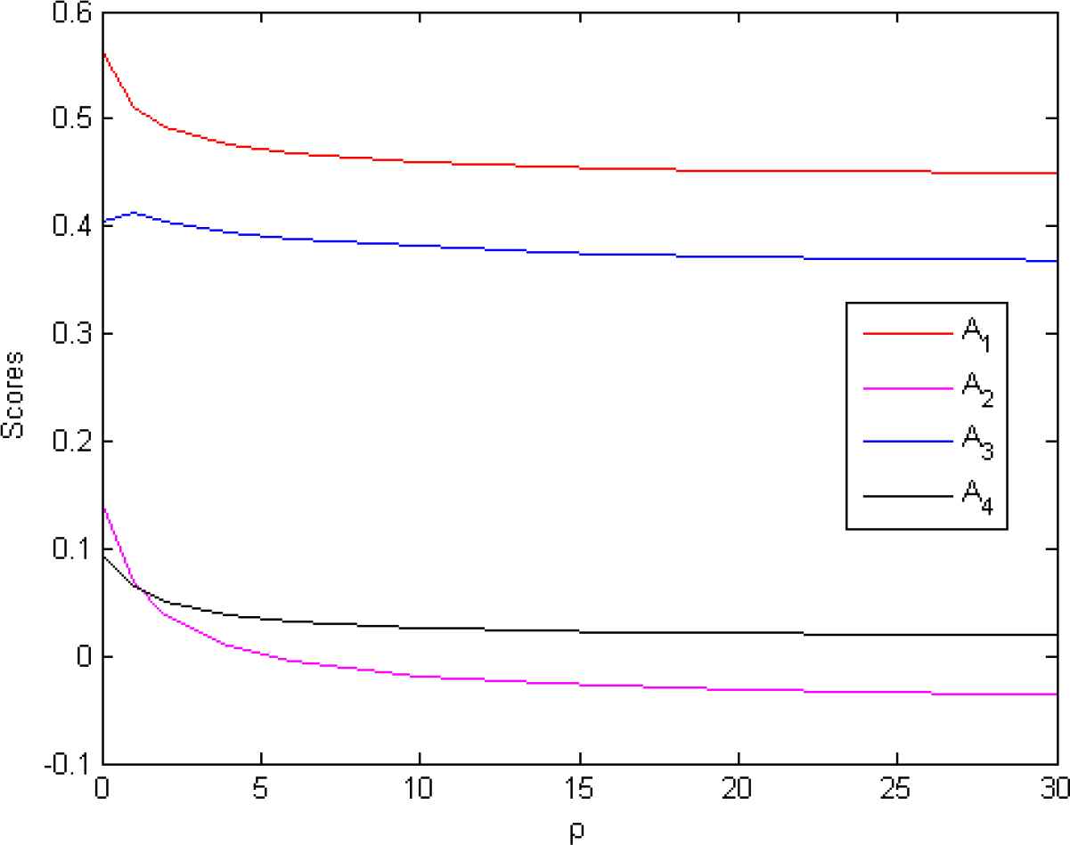
Scores for alternatives determined using the Hamacher Pythagorean fuzzy interactive weighted averaging (HPFIWA) operator.

Figure 2

Scores for alternatives determined using the Hamacher Pythagorean fuzzy interactive weighted geometric (HPFIWG) operator.

From Figure 1, we can obtain that the scores determined by the HPFIWA operator of alternative A3 first increases and then decreases as the value ρ increase,the reason is that the score function of alternative A3 is a monotone increasing function about parameter ρ in interval [0,0.4097] and a monotone decreasing function about parameter ρ in interval (0.4097,30], whereas the scores of other alternatives determined by the HPFIWA operator decrease as the value ρ increase. Since the parameter ρ is smaller, the score values of all alternatives are larger, then for an optimistic DM, smaller ρ is advised. Further analysis, we can get the following results:

  1. When ρ(0,1.2275], the ranking is A1A3A2A4.

  2. When ρ(1.2275,30], the ranking is A1A3A4A2.

As shown in Figure 2, the scores determined employing the HPFIWG operator of alternative A2 increase as the value ρ increase, whereas the scores of other alternatives derived from the HPFIWG operator first decrease and then increase when the value ρ increase. Because the parameter ρ is bigger, the score values of all alternatives are larger, then as an optimistic DM, bigger ρ is advised. Further analysis, we can get the following results:

  1. When ρ(0,11.8182], the ranking is A1A3A2A4.

  2. When ρ(11.8182,30], the ranking is A3A1A4A2.

Furthermore, if the HPFIWA and HPFIWG operators are replaced respectively with FPFIWA and FPFIWG operators to resolve above example, then the score outcomes with the change of parameter ε are described in Figures 3 and 4, respectively.

Figure 3

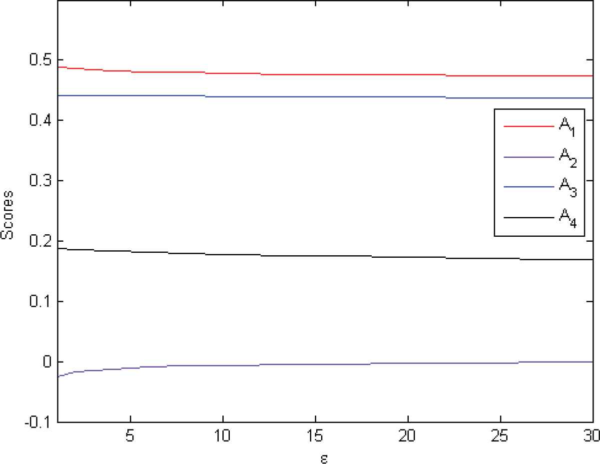
Scores for alternatives determined using the Frank Pythagorean fuzzy interactive weighted averaging (FPFIWA) operator.

Figure 4

Scores for alternatives determined using the Frank Pythagorean fuzzy interactive weighted geometric (FPFIWG) operator.

In the light of Figure 3, we can get that the scores acquired via the FPFIWA operator of alternative A4 first decreases and then increases as the value ε increases, whereas the scores of other alternatives determined utilizing the FPFIWA operator decrease when the value ε increases. Because the parameter ε is smaller, the score values of all alternatives are larger, then as an optimistic DM, smaller ε is advised. Further research, the following results can be obtained:

  1. When ε(0,1.4185], the ranking is A1A3A2A4.

  2. When ε(1.4185,30], the ranking is A1A3A4A2.

Based on Figure 4, we notice that the scores generated via the FPFIWG operator of alternatives A1 and A4 decrease when the value ε increases, whereas the changing trend of scores for alternative A2 is just the opposite of alternatives A1 and A4. The scores acquired using the FPFIWG operator of alternative A3 first increases and then decreases when the value ε increases. And regardless of the scores of the four alternatives change, the ranking results are always the same, that is A1A3A4A2.

6.3.3. Comparative analysis with the relevant approaches

In order to show the effectives and merits of proposed approach (As mentioned above, we select HPFIWA and HPFIWG operators to stand for the proposed AOs), we will compare with the following methods: Ma and Xu's method [22] based on PFWA operator, Garg's method [24] based on PFEWA operator, Wu and Wei's method [27] based on PFHWA operator, Wei's method [32] based on PFIWA operator, Gao et al.'s method [37] based on PFIPWA operator and Wang and Li's method [38] based on WPFIPBM operator. The evaluation values in Table 1 are employed, and the comparison results are provided in Table 4.

Approaches Score Value s(yi) Ranking
Ma and Xu's method [22] based on PFWA operator s(y1)=0.5223,s(y2)=0.1354,s(y3)=0.5910,s(y4)=0.2337 A3A1A4A2
Garg's method [24] based on PFEWA operator s(y1)=0.5080,s(y2)=0.1059,s(y3)=0.5844,s(y4)=0.2075 A3A1A4A2
Wu and Wei's method [27] based on PFHWA operator s(y1)=0.5008,s(y2)=0.0916,s(y3)=0.5802,s(y4)=0.1948 A3A1A4A2
Wei's method [32] based on PFIWA operator s(y1)=0.5110,s(y2)=0.0686,s(y3)=0.4127,s(y4)=0.0648 A1A3A2A4
Gao et al.'s method [37] based on PFIPWA operator s(y1)=0.5060,s(y2)=0.0534,s(y3)=0.4207,s(y4)=0.0626 A1A3A4A2
Wang and Li's method [38] based on WPFIPBM operator (p=q=1) s(y1)=0.4981,s(y2)=0.0719,s(y3)=0.4780,s(y4)=0.1887 A1A3A4A2
Proposed method based on HPFIWA operator (ρ=3) s(y1)=0.4822,s(y2)=0.0200,s(y3)=0.3998,s(y4)=0.0429 A1A3A4A2
Proposed method based on HPFIWG operator (ρ=3) s(y1)=0.4836,s(y2)=0.0051,s(y3)=0.4517,s(y4)=0.1973 A1A3A4A2
Table 4

The aggregating results by different approaches.

This Table reveals that the ranking outcomes utilizing the presented method are same with the methods defined by [32,37,38], which indicates that our novel proposed approach is valid. Moreover, the ranking outcomes are different from the methods given by [22,24,27]. Further discussions are listed as follows:

  1. Ma and Xu's method [22] is on the base of PFWA operator, the PFWA operator adopted the algebra t-conorm and t-norm, it is a particular form of ATT. Although the calculation process is relatively easy, it cannot capture the interaction over MD and NMD of PFNs. Hence the ranking output by Ma and Xu's method [22]is different from our defined method.

  2. Garg's method [24] and Wu and Wei's method [27] are based on the PFEWA and PFHWA operators, respectively. The PFEWA operator adopted the Einstein t-conorm and t-norm, and the PFHWA operator adopted the Hamacher t-conorm and t-norm. Whereas, the presented method used the ATT, and Einstein t-conorm and t-norm, Hamacher t-conorm and t-norm are all special cases of ATT. On the other hand, like Ma and Xu 's method [22], the methods[24,27] also do not reflect the interactive influence among MD and NMD, so the ranking outputs by these two methods [24,27] are different from our constructed method. It reveals the superiority of our built method.

  3. Wei's method [32] is based on PFIWA operator, which is the special case of proposed HPFIWA operator, when the function l(r) takes log(r).

  4. Gao et al.'s method [37] is on the basis of PFIPWA operator, which can reduce the impact of confused data during the aggregation process. Although the PFIPWA operator can capture the interactive influence over MD and NMD, but it utilizes algebra t-conorm and t-norm.

  5. Wang and Li's method [38] is based on WPFIPBM operator, to settle above MADM issue, we take the valued p=q=1, and then decision result coincides with the presented HPFIWA operator. It displays that the effectiveness of our defined AOs. But the superiority of our built method is that it uses ATT, so it is more flexible.

Figure 5

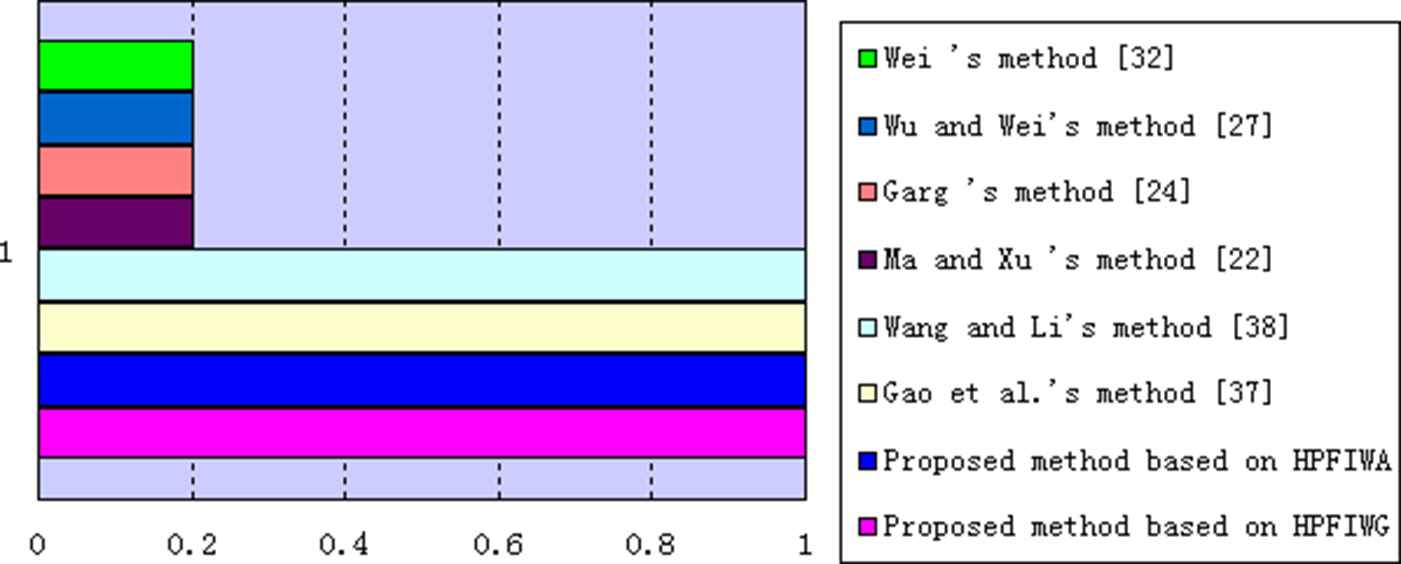
Spearman correlation: presented methods versus others.

As shown in Figure 5, the spearman's coefficient of proposed method (HPFIWA, HPFIWG), Gao et al.'s method [37] and Wang and Li's method [38] are all 1, which reveals the validity of the explored method. Furthermore, the spearman's coefficient of Ma and Xu's method [22], Garg's method [24], Wu and Wei’s method [27] and Wei’s method [32] are all 0.2, which indicates the superiority of the constructed method.

In a word, the superiorities of our explored method are summarized as follows: (1) It can offer a more flexible method via selecting diverse forms of ATT; (2) It can reflect the interactive influence among MD and NMD for PFNs in the decision-making process.

7. CONCLUSION

ATT can derive many famous t-conorms and t-norms, PFS is a remarkable technique to depict the fuzziness and indeterminacy in MADM issues. In this study, we have constructed several novel interactive operational rules for PFNs in the light of ATT, based on which, some novel interactive AOs are explored, they are A-PFIWA operator and A-PFIWG operator. In addition, we discussed their properties, such as their idempotency, monotonicity boundedness, shift-invariance and so on. When the parameter varies in the presented AOs, we acquire certain specific Pythagorean fuzzy interactive AOs. Further, we have provided a decision-making approach for MADM issue on the basis of these AOs. Finally, an actual issue on assessment of online payment service providers is settled to show the availability of presented approach, meanwhile, a detailed investigation are also provided with respect to the change trend of decision results when the parameter varies in introduced AOs. Furthermore, the superiority of built approach is given by comparing to relevant approaches. The shortcomings of the operators proposed in this paper are that: (1) They do not consider the interrelationship between the input PFNs; (2) The aggregated result is relatively complicated by using the proposed operators.

In the succeeding research, we shall extend the constructed approach to other applications [5158], or study the parameter determination of Bonferroni operators [59] and also extend to proportional interval type-2 hesitant fuzzy set [60].

CONFLICTS OF INTEREST

The authors declare no conflict of interests regarding the publication for the paper.

AUTHORS' CONTRIBUTIONS

L.W. (LeiWang) conceived this work, L.W. and H.G. (Harish Garg) compiled the computing program by Matlab and analyzed the data, L.W. and H.G. wrote the paper. Finally, all the authors have read and approved the final manuscript. All authors have read and agreed to the published version of the manuscript.

ACKNOWLEDGMENTS

The authors are very grateful to the anonymous reviewers for their valuable comments and constructive suggestions that greatly improved the quality of this paper. The work was partly supported by the Scientific Research Funds Project of Liaoning Province Education Department (No. LJ2019QL014; No. LJ2020JCL018).

REFERENCES

41.G. Klir and B. Yuan, Fuzzy Sets and Fuzzy logic: Theory and Applications, Prentice Hall, Upper Saddle River, NJ, 1995.
42.H.T. Nguyen and E.A. Walker, A First Course in Fuzzy Logic, CRC Press, Boca Raton, Florida, 1997.
49.E.P. Klement and R. Mesiar, Logical, Algebraic, Analytic, and Probabilistic Aspects of Triangular Norms, Elsevier, New York, 2005.
Journal
International Journal of Computational Intelligence Systems
Volume-Issue
14 - 1
Pages
503 - 527
Publication Date
2020/12/24
ISSN (Online)
1875-6883
ISSN (Print)
1875-6891
DOI
10.2991/ijcis.d.201215.002How to use a DOI?
Copyright
© 2021 The Authors. Published by Atlantis Press B.V.
Open Access
This is an open access article distributed under the CC BY-NC 4.0 license (http://creativecommons.org/licenses/by-nc/4.0/).

Cite this article

TY  - JOUR
AU  - Lei Wang
AU  - Harish Garg
PY  - 2020
DA  - 2020/12/24
TI  - Algorithm for Multiple Attribute Decision-Making with Interactive Archimedean Norm Operations Under Pythagorean Fuzzy Uncertainty
JO  - International Journal of Computational Intelligence Systems
SP  - 503
EP  - 527
VL  - 14
IS  - 1
SN  - 1875-6883
UR  - https://doi.org/10.2991/ijcis.d.201215.002
DO  - 10.2991/ijcis.d.201215.002
ID  - Wang2020
ER  -