A. Differential Evolution

DE [26] is a very competitive optimizer for optimization problems. The key steps of DE algorithm are initialization, mutation, crossover, and selection, which are briefly introduced below.

1. Initialization: For an optimization problem of dimension D, a population x of NP real-valued vectors (or individuals) is typically initialized at random in accordance with a uniform distribution in the search space S. The jth decision variable of the ith individual at generation g can be initialized as follows:

   xi,j,g=Lj+rand×Uj−Lj,i=1,⋯,NP,j=1,⋯,D (3)
   where L_j and U_j are the lower and upper bounds of jth dimension, respectively. rand represents a uniformly distributed random number in the range of (0,1).

2. Mutation: In each generation, a mutant vector is formed for each individual based on scaled difference individuals. The frequently used mutation operators are listed below.

   “DE/rand/1”

   vi,G=xr1,G+Fxr2,G−xr3,G(4)

   “DE/best/1”

   vi,G=xbest,G+Fxr1,G−xr2,G (5)

   “DE/rand/2”

   vi,G=xr1,G+Fxr2,G−xr3,G+Fxr4,G−xr5,G(6)

   “DE/best/2”

   vi,G=xbest,G+Fxr1,G−Xr2,G+Fxr3,G−xr4,G(7)

   “DE/current-to-best/1”

   vi,G=xi,G+Fxbest,G−xi,G+Fxr1,G−xr2,G (8)

   “DE/current-to-rand/1”

   vi,G=xi,G+Kxr1,G−xi,G+F′xr2,G−xr3,G (9)
   where i = 1,…,NP, r₁, r₂, r₃ϵ{1,…,NP} are randomly selected and satisfy r₁≠r₂≠r₃≠i, Fϵ[0,1], F is control parameter. In “DE/current-to-rand/1,” K is the combination coefficient, which should be chosen with a uniform random distribution from [0, 1] and F’ = K•F.

3. Crossover: DE employs a binomial crossover operation on the target vector x_i and the mutant vector v_i to form a trial vector u_i as follows:

   ui,Gj=vi,Gjif(randj(0,1)≤Crorj=jrand)xi,Gj,otherwisej=1,2,…,D(10)
   where j_rand is randomly selected from [1, D] to ensure that the trial vector has at least one dimension differ from the target vector. Cr is the crossover rate lying in the range of [0, 1].

4. Selection: The selection operator is employed to decide which one is to survival in the next generation through a one-to-one competition between the target vector and its trial vector. Take the maximization optimization problem as an example, the selection process can be outlined as

   xi,G+1=ui,G, iffui,G≥fxi,Gxi,G, otherwise(11)
   where f⋅ is the objective function to be optimized (maximized).

As mentioned before, DE or other EAs have been employed for multimodal optimization. However, it is difficult for the algorithms to locate all the global optima in a run. On the one hand, the algorithm should maintain sufficient diversity to ensure the individuals to spread out widely within the search space. On the other hand, the individuals gather around potential local optima to fully exploit each optimum region. Therefore, it is greatly desirable for DE or other EAs to make a balance between exploration (diversity) and exploitation (convergence).

B. Niching Techniques for Multimodal Optimization

Niching is a concept derived from biology and refers to a living environment. The species evolve in different living environments. In terms of MMOP, niching refers local regions around an optimum. A brief review of representative niching techniques is given in the following.

The crowding strategy proposed by De Jong is one of the simplest niching techniques for MMOPs. The advantage of this strategy is that it can maintain the diversity of the whole population. However, the potential optimal solution will be replaced if the offspring is a superior solution. This phenomenon is called replacement error. To overcome this problem, deterministic crowding and probabilistic crowding, two improvement strategies to the original crowding, are proposed [11,27]. The deterministic crowding can effectively reduce replacement errors, while probabilistic crowding can prevent the loss of niches with lower fitness or loss of local optima. Nevertheless, the disadvantage of probabilistic crowding is slow convergence and poor fine searching ability. The restricted tournament selection (RTS) employs Euclidean or Hamming distance to find the nearest member within the w (window size) individuals. Similar to crowding, RTS can ensure the population diversity by the competition between similar individuals. However, this strategy suffers from the replacement error.

Both the fitness sharing strategy and speciation employ the grouping method. More precisely, the population is divided into different sub-populations according to the similarity of the individuals. The advantage of fitness sharing strategy is the stable niches maintained. However, the niche radius σshare and rs used in sharing and speciation, respectively, are difficult to specify for lacking of prior knowledge of the problems. Moreover, the computational complexity of sharing is much expensive.

In order to improve the niching techniques mentioned above, the neighborhood base CDE (NCDE) and the neighborhood based SDE (NSDE) are proposed in [2]. However, a new parameter m, which is the neighborhood size, is introduced in NCDE and NSDE. In order to relieve the influence of the parameter, Biswas et al. [28] introduced an improved local information sharing mechanism in niching DE, where the neighborhood size is dynamically changed in a nonlinear way. Shir et al. [25] proposed a niching variant of the covariance matrix adaptation evolution strategy (CMA-ES), where a technique called dynamic peak identification (DPI) is used to split the population into species. The number of niches, that is, the number of peaks of optimization problem, is predefined in DPI. However, it is practically difficult to know in advance the number of peaks that exist within the landscape of optimization problem.

C. Novel Operators for Multimodal Optimization

Wang et al. [29] introduced a dual-strategy mutation scheme in DE to balance exploration and exploitation in generating offspring. Moreover, in order to select suitable individuals from different clusters, an adaptive probabilistic selection mechanism based on affinity propagation clustering is proposed. In order to eliminate the requirement of prior knowledge to specify certain niching parameters, Qu et al. [14] proposed a distance-based locally informed particle swarm (LIPS) optimizer. LIPS employs the Euclidean-distance-based neighborhood information to guide the search process. Therefore, LIPS is able to form different stable niches and locate the desired peaks with high accuracy. However, the neighborhood size that influences the performance of the proposed LIPS is difficult to exactly specify. A larger neighborhood size is suitable for convergence while a smaller neighborhood size is suitable for maintaining the diversity of the population. To achieve a balance between local exploitation and global exploration with speciation niching technique, Hui et al. [30] proposed an ensemble and arithmetic recombination-based speciation differential evolution algorithm (EARSDE), in which the arithmetic recombination is used to enhance exploration and the neighborhood mutation is employed to improve exploitation of individual peaks. Haghbayan et al. [3] proposed an improved niching strategy which employs a nearest neighbor scheme and hill valley algorithm to control the interaction between GSA agents. Fieldsend et al. [31] proposed the niching migratory multi-swarm optimizer (NMMSO) which dynamically manages many particle swarms. In NMMSO, multiple swarms which have strong local search continuously merge and split in the search landscape. More precisely, the swarms will split if new regions are identified. In addition, they merge to prevent duplication of labor. Li [22] proposed RPSO (including r2PSO and r3PSO) by employing ring topology which using individual particles’ local memories to form a stable network. The network can retain the best particles which explore the search space more broadly.

D. Multiobjective Optimization Techniques for Multimodal Optimization

Similar to MOPs, a MMOP involves multiple optimal solutions. Therefore, a few attempts have been made to solve MMOPs by taking advantage of multiobjective optimization in maintaining good population diversity. For instance, Wang et al. [13] proposed a novel transformation technique MOMMOP which transforms an MMOP into an MOP with two conflicting objectives. Moreover, MOMMOP finds a trade-off between exploitation and exploration by balancing the decision variable and the objective function. Basak et al. [32] brought up a novel bi-objective formulation of the MMOP, in which the mean distance-based selection mechanism is chosen as the second objective to prevent the entire population from converging to a single optimum. Yao et al. [17] proposed a bi-objective multipopulation generic algorithm which employs a novel bi-objective mechanism and a multipopulation scheme to realize exploration. Therefore, the sub-populations of BMPGA are evolved toward two objectives separately and simultaneously instead of toward a single fitness objective. Li [33] introduced a multiobjective optimization method into the matrix adaptation evolution strategy (MA-ES) to solve MMOPs.

A. Framework of BMDE

The main framework of the proposed BMDE is summarized in Algorithm 1, from which we can see that BMDE is composed of three main strategies: (1) bi-population strategy; (2) multi-mutation strategy; and (3) update strategy. In bi-population evolution strategy, one population consists of the individuals with higher fitness value is employed for exploitation, while the other population which consists of the individuals with lower fitness value is used for exploration. Then, a multi-mutation strategy is employed to improve the solution accuracy and find more optimal solutions. Finally, update strategy is performed to generate new individuals to replace those with high similarity. The following sections will detail the three main strategies in Algorithm 1 successively.

B. Multi-Mutation Strategy

DE has been proved to be an efficient algorithm in the past two decades due to its powerful global optimization properties on a wide range of problems, and its simplicity [34]. Here, we exploit the DE algorithm for multimodal optimization. As mentioned before, there are several widely used mutation strategies of DE. Different mutation strategies have different characteristics. DE/rand/1 and DE/rand/2 have a high diversity to avoid premature convergence. However, their convergence rate is poor. DE/best/1 and DE/best/2 perform better in convergence rate, however, they are easy to be trapped in local minima. As for DE/current-to-best/1 or DE/current-to-rand/1, it can be employed as a mixed strategy that combines a current individual and a best individual (or a rand individual) as the origin individual and the terminal individual, respectively to form a composite base vector [30]. DE/current-to-best/1 and DE/current-to-rand/1 can escape from local minima with better diversity than DE/best/1 and DE/best/2.

As shown previously, niching is an effective technique to locate multiple optima in parallel. However, most niching methods have difficulties that need to be overcome [22], such as reliance on prior knowledge of some niching parameters, difficulty in maintaining found solutions in a run, higher computational complexity, etc. Inspired from the aforesaid observations in DE, we employ a multi-mutation strategy that utilizes two different mutation strategies instead of utilizing niching technique. One mutation strategy is DE/rand/1 which has a high diversity to avoid premature convergence. The other mutation strategy is developed based on DE/current-to-rand/1 and fitness Euclidean-distance ratio [21] which encourages the survival of fitter and closer individuals, denoted as DE_FER. The mutation strategy DE_FER can be calculated as follows:

where rand_i,G of ith individual is a uniform random distribution from [0, 1]. In order to search for multiple peaks, instead of using a single global best at generation G, each individual is attracted toward x_fer,G, a fittest-and-closest neighborhood individual, which is achieved via computing its fitness and Euclidean-distance ratio. The fitness and Euclidean-distance ratio of x_i,G is described as follows [21]: where NP is the population size. f(•) is the objective (fitness) function to be optimized (maximized). ||•||₂ is Euclidean-distance of two individuals. η is a scaling factor to avoid fitness and Euclidean distance dominating each other. where L and U denote the lower bound and upper bound of the search space of D dimension, respectively. x_best and x_worst are the best-fit individual and the worst-fit individual in the current generation, respectively.

The index (fer) corresponding to the maximum value of FER is defined by

The multi-mutation strategy is described in Algorithm 2. NP is the population size. δ=1D+modD,2, D is the dimension, and mod(•) is modular operation.

Multi-mutation strategy is able to keep a balance between the exploration and exploitation, which make it suitable for multimodal problem. DE/rand/1 uses the rand vector selected from the population to generate donor vectors. The scheme promotes exploration since all the vectors/individuals are attracted toward different position in the search space through iterations, thereby ensuring the population diversity. DE_FER uses the local best vector, i.e., a fittest-and-closest neighborhood individual. The local best vector can guide other vectors/individuals to exploit, so as to enhance local search ability.

C. Bi-population Evolution Strategy

Diversity and convergence are two targets that need to be achieved for dealing with MMOPs efficiently. As evolution progresses, the individuals with higher fitness tend to attract other inferior individuals, thereby inducing hill climbing behavior [34]. On the one hand, this behavior leads to loss of some peaks because of selection pressure and genetic drifts. On the other hand, as the research in [19] pointed out, historical data is another source that can be used to improve the algorithm performance. Hence, we are interested in a set of recently explored inferior individuals which may be used as a promising direction toward the optimum.

Motivated by this observation, instead of employing a single population in conventional DE, we use bi-population to achieve a good balance between locating different peaks by exploring and improving the solution precision by exploiting. Here, we denote FP as the evolution population to save the individuals who win in the competition and denote SP as the inferior population to save the individuals who fail in the competition. First, SP is initiated to be empty. For each offspring u_i, we calculate the Euclidean distance of u_i to the individuals in the current population. Then, the minimum Euclidean distance is calculated as follows:

where j′ is the index of the nearest individual to the offspring u_i. L and U denote the lower bound and upper bound of the search space, respectively.

Compare the fitness of the offspring u_i and the individual x_j′, if u_i is more fit than x_j′, the superior individual u_i will replace x_j′ in the population FP. Meanwhile, if the Euclidean distance between two individuals is greater than σ, the worse individual x_j′ will be saved in the population SP. If the size of SP (denotes as |SP|) is larger than k times the population size NP, the (|SP|−k×NP) worst-ranking individuals are deleted from the population. The bi-population evolution strategy is described in Algorithm 3. σ is set to 0.01, which is based on a large number of experiments.

Bi-population evolution strategy employs two populations to perform multimodal optimization in parallel. One the one hand, the difference between inferior individuals and the current individuals can be considered as a promising direction toward the optimum. Therefore, inferior population can be employed to improve the population diversity and explore more peaks. On the other hand, evolution population that consists of superior individuals have good fitness, which can exploit the region around the superior individuals to accelerate the convergence speed.

D. Update Strategy

During the evolution process, the individuals are attracted toward the superior individuals. After several generations of evolution, many individuals may have high similarity because of selection pressure. These individuals may explore the same peak. Obviously, this is a waste of resources. In addition, if the number of individuals surrounded a peak is too small, this behavior may lead to loss of the peak. As a result, it is difficult for the algorithm to find as many distinct global peaks as possible. Therefore, the proposed algorithm eliminates the individuals which have high similarity and generates new individuals to enhance the population diversity.

The location (U) of updated individual is calculated as follows:

The setting of σ is the same as that of σ in Algorithm 4.

For all updated individuals (u∈U), the mutation strategy can be calculated as follows:

where x_r1,G, x_r2,G are randomly selected from the current population and satisfy r₁≠r₂, while x~r3,G is randomly selected from the inferior population SP.

The pseudocode of the population updating is shown in Algorithm 4.

E. Complexity Analysis

The computational cost of BMDE mainly comes from the multi-mutation strategy, bi-population evolution strategy, and update strategy. For multi-mutation strategy, a loop over NP (population size) is conducted, containing a loop over D (dimension). The mutation and crossover operations are performed at the component level for each individual. Then, the runtime complexity is ONP⋅D at each iteration. For bi-population evolution strategy, first, we need to compare the objective function values of the offspring u_i and its nearest individual x_j’ in order to save better individual. Next, if the Euclidean distance between u_i and x_j’ is greater than the given threshold, the worse individual x_j’ will be saved in the inferior population. Hence in the worst possible case, the runtime complexity is O2⋅NP at each iteration. For update strategy, in the worst possible case, if there are m (m < NP) individuals to be updated, the runtime complexity is Om⋅NP⋅D at each iteration. The total time complexity of BMDE at one iteration can be estimated as follows:

Therefore, the time complexity of the proposed algorithm is ONP⋅D.

A. Benchmark Functions

In this section, 20 widely used benchmark functions from CEC2013 [20] test suite are employed to verify the effectiveness of the proposed algorithm against other state-of-the-art algorithms. These functions can be divided into two groups. This first group includes F₁–F₁₀ which are simple and low-dimensional multimodal problems. F₁–F₅ have a small number of global optima, and F₆–F₁₀ have a large number of global optima. The second group includes F₁₁–F₂₀ which are composition multimodal problems composed of several basic problems with different characteristics. These benchmark functions show some characteristics like uneven landscape, multiple global optima and local optima, unequal spacing among optima, etc. The properties of these functions are given in Table 1. The meaning of each column is as follows. r denotes the niche radius. D denotes the dimension of the test function. The fourth column denotes the number of global optimal solutions for each test function. In order to ensure a fair comparison between the compared algorithms, the algorithm will terminate when the number of function evaluations reaches the specified threshold. MaxFES denotes the values of the maximum number of function evaluations (MaxFES) for each compared algorithm. The last column represents the population size for each function to be optimized.

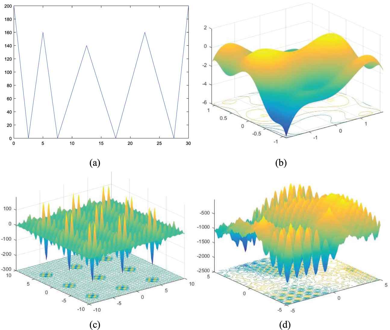
Some functions from the CEC2013 are drawn in the following. Five-Uneven-Peak Trap (F₁) has 2 global optima and 3 local optima, as shown in Figure 1 (a). Six-Hump Camel Back function (F₅) has 2 global optima and 2 local optima, as shown in Figure 1(b). Figure 1(c) shows an example of the Shubert 2D function (F₆), where there are 18 global optima in 9 pairs. Figure 1 (d) shows the 2D version of CF₂ (F₁₂). Composition Function 2 (CF₂) is constructed based on eight basic functions, therefore it has eight global optima. The basic functions used in CF₂ include Rastrigin’s function, Weierstrass function, Griewank’s function, and Shpere function.

Figure 1

Four functions from the Congress on Evolutionary Computation 2013.

B. Algorithms Compared

In this paper, 13 algorithms are selected to compare with the proposed algorithm. These algorithms can be divided into four categories. CDE, FERPSO, r2PSO, r3PSO, r2PSO-lhc, r3PSO-lhc, NCDE, SCMA-ES, and MA-ESN belong to the category of niching without niching parameters. SDE and NSDE belong to the category of speciation. NShDE belongs to the category of fitness sharing. MOMMOP belongs to the category of using multiobjective optimization method for MMOPs. The state-of-the-art multimodal algorithms used for comparison with BMDE are shown as follows.

1. CDE [11]: Crowding DE.

2. SDE [2]: Species DE.

3. FERPSO [21]: fitness-Euclidean-distance ration PSO.

4. r2PSO [22]: lbest PSO that interacts to its immediate right member by using a ring topology.

5. r3PSO [22]: lbest PSO that interacts to its immediate left and right member by using a ring topology.

6. r2PSO-lhc [22]: r2PSO model without overlapping neighborhoods.

7. r3PSO-lhc [22]: r3PSO model without overlapping neighborhoods.

8. NSDE [2]: neighborhood based SDE.

9. NShDE [2]: neighborhood based sharing DE.

10. NCDE [2]: neighborhood based CDE.

11. MOMMOP [13]: multiobjective optimization for MMOPs

12. SCMA-ES [23]: self-adaptive niching CMA-ES

13. MA-ESN [24–25]: matrix adaptation evolution strategy with dynamic niching

14. BMDE: the proposed algorithm.

C. Experimental Platform and Parameter Setting

To obtain an unbiased comparison, all the experiments are carried out on the same machine with an Intel Core i7-3770 3.40 GHz CPU and 4 GB memory.

All the algorithms use the same termination criterion, i.e., the MaxFES. The settings of MaxFES for the test functions are shown in Table 1. Each algorithm is run 25 times for each test function. The population size of BMDE is described in Table 1. The population size of other algorithms agree well with the original papers. Other parameter settings of each algorithm are provided in Table 2.

Generally, there are five accuracy thresholds, ε = 1.0E–1, ε = 1.0E–2, ε = 1.0E–3, ε = 1.0E–4, and ε = 1.0E–5. ε = 1.0E–1 and ε = 1.0E–2 are easily available. Therefore, the accuracy thresholds with ε = 1.0E–3, ε = 1.0E–4, and ε = 1.0E–5 are selected in the experiments. In addition, two well-known criteria [11] called peak ratio (PR) and success rate (SR) are employed to measure the performance of different multimodal optimization algorithms for each function. PR denotes the average percentage of all known global optima found over all runs, while SR denotes the percentage of successfully detecting all global optima out of all runs for each function.

In view of statistics significance of the results, the Wilcoxon signed-rank test [35] at the 5% significance level is employed to compare BMDE with other compared algorithms. “≈,” “−,” and “+” are applied to express the performance of BMDE is similar to (≈), worse than (−), and better than (+) that of the compared algorithm, respectively. Moreover, the Friedman’s test, which is implemented by using KEEL software [36], is used to determine the ranking of all compared algorithms.

D. Comparisons with State-of-the-Art Multimodal Algorithms

Tables 3–5 show the result obtained by BMDE, CDE, SDE, FERPSO, r2PSO, r3PSO, r2PSO-lhc, r3PSO-lhc, NSDE, NShDE, NCDE, MOMMOP, SCMA-ES, and MA-ESN on F₁−F₁₀ with respect to PR and SR at three accuracy levels, i.e., ε = 1.0E−3, ε = 1.0E−4, and ε = 1.0E−5. For the functions F₁−F₁₀, as can be seen from Tables 3–5, BMDE can find all global solutions in a single run at three accuracy levels.

Table 3 shows that BMDE performs better than SDE, r2PSO, r2PSO-lhc on F₁, F₄, F₆, F₇, F₈, F₉ and F₁₀. BMDE performs better than CDE on F₄, F₆, F₇, F₈, and F₉. BMDE performs better than FERPSO and r3PSO-lhc on F₁, F₆, F₇, F₈, F₉, and F₁₀. BMDE performs better than r3PSO on all problems except F₃ and F₅. BMDE performs better than NSDE on F₄, F₆, F₇, F₈, F₉^, and F₁₀. BMDE performs better than NShDE on F₆, F₇, F₈, F₉, and F₁₀. BMDE performs better than NCDE on F₆, F₇, F₈, and F₉. BMDE performs better than SCMA-ES and MA-ESN on all problems except F₁. MOMMOP can find all global solutions in a single run at ε = 1.0E−3. BMDE outperforms CDE, SDE, FERPSO, r2PSO, r3PSO, r2PSO-lhc, r3PSO-lhc, NSDE, NShDE, NCDE, MOMMOP, SCMA-ES, and MA-ESN on 5, 7, 6, 6, 7, 6, 6, 5, 5, 2, 0, 9, 9 test problems, respectively.

Table 4 indicates that BMDE performs better than SDE, r2PSO, r2PSO-lhc, r3PSO-lhc on F₁, F₄, F₆, F₇, F₈, F₉, and F₁₀. BMDE performs better than CDE on F₄, F₆, F₇, F₈, and F₉. BMDE performs better than FERPSO on F₁, F₆, F₇, F₈, F₉, and F₁₀. BMDE performs better than r3PSO on all problems except F₃ and F₅. BMDE performs better than NSDE on F₄, F₆, F₇, F₈, F₉, and F₁₀. BMDE performs better than NShDE and NCDE on F₆, F₇, F₈, F₉, and F₁₀. BMDE performs better than MOMMOP on F₄ and F₉. BMDE performs better than SCMA-ES and MA-ESN on all problems except F₁. BMDE outperforms CDE, SDE, FERPSO, r2PSO, r3PSO, r2PSO-lhc, r3PSO-lhc, NSDE, NShDE, NCDE, MOMMOP, SCMA-ES, and MA-ESN on 5, 7, 6, 7, 7, 7, 6, 6, 5, 3, 0, 9, 9 test problems, respectively.

Table 5 indicates that BMDE performs better than SDE, FERPSO, r2PSO, r2PSO-lhc, on F₁, F₄, F₆, F₇, F₈, F₉, and F₁₀. BMDE performs better than CDE on F₄, F₆, F₇, F₈, and F₉. BMDE performs better than r3PSO on all problems except F₃ and F₅. BMDE performs better than r3PSO-lhc on all problems except F₂ and F₃. BMDE performs better than NSDE on F₄, F₅, F₆, F₇, F₈, F₉, and F₁₀. BMDE performs better than NShDE and NCDE on F₆, F₇, F₈, F₉, and F₁₀. BMDE performs better than MOMMOP on F₄ and F₉. BMDE performs better than SCMA-ES and MA-ESN on all problems except F₁. BMDE outperforms CDE, SDE, FERPSO, r2PSO, r3PSO, r2PSO-lhc, r3PSO-lhc, NSDE, NShDE, NCDE, MOMMOP, SCMA-ES, and MA-ESN on 5, 7, 6, 7, 7, 7, 7, 6, 5, 4, 1, 9, 9 test problems, respectively.

Tables 6–8 shows the result obtained by BMDE, CDE, SDE, FERPSO, r2PSO, r3PSO, r2PSO-lhc, r3PSO-lhc, NSDE, NShDE, NCDE, MOMMOP, SCMA-ES, and MA-ESN on F₁₁−F₂₀ with respect to PR and SR at ε = 1.0E−3, ε = 1.0E−4, and ε = 1.0E−5, respectively. As can be seen in Tables 6–8, BMDE performs better than CDE, SDE, r2PSO, r3PSO, r2PSO-lhc, r3PSO-lhc, and NSDE on all problems at ε = 1.0E−3, ε = 1.0E−4, and ε = 1.0E−5, respectively. BMDE performs better than FERPSO on all problems except F₁₂ at three accuracy levels. BMDE performs better than NShDE on F₁₁, F₁₂, F₁₃, F₁₅, F₁₆, F₁₈, and F₁₉at ε = 1.0E−5. BMDE performs better than NCDE on all problems except F₂₀ at ε = 1.0E−4 and ε = 1.0E−5, respectively. BMDE performs better than MOMMOP on F₁₁, F₁₃, and F₁₆ at ε = 1.0E−4 and ε = 1.0E−5, respectively. BMDE performs better than SCMA-ES and MA-ESN on all problems except F₁₉ at three accuracy levels.

BMDE outperforms CDE, SDE, FERPSO, r2PSO, r3PSO, r2PSO-lhc, r3PSO-lhc, NSDE, NShDE, NCDE, MOMMOP, SCMA-ES, and MA-ESN on 10, 10, 8, 10, 10, 10, 10, 10, 4, 4, 1, 9, 9 test problems at ε = 1.0E−3, respectively. BMDE outperforms CDE, SDE, FERPSO, r2PSO, r3PSO, r2PSO-lhc, r3PSO-lhc, NSDE, NShDE, NCDE, MOMMOP, SCMA-ES, and MA-ESN on 10, 10, 8, 10, 10, 10, 10, 10, 4, 6, 2, 9, 9 test problems at ε = 1.0E−4, respectively. BMDE outperforms CDE, SDE, FERPSO, r2PSO, r3PSO, r2PSO-lhc, r3PSO-lhc, NSDE, NShDE, NCDE, MOMMOP, SCMA-ES, and MA-ESN on 10, 10, 8, 10, 10, 10, 10, 10, 4, 7, 2, 9, 9 test problems at ε = 1.0E−5, respectively.

Tables 3–8 show that the number of “+ (better)” obtained by the proposed algorithm is bigger than most compared algorithms except MOMMOP. It was experimental shown that BMDE ranks first among all algorithms when accuracy level ε = 1.0E−5, while BMDE ranks second among all algorithms when accuracy level ε = 1.0E−3 and ε = 1.0E−4. Apart from MOMMOP, the average excellent and good rate of BMDE for 20 functions is 73.75% (∑i=120bi/(20×12)) when ε = 1.0E−3, the average excellent and good rate of BMDE is 76.25% (∑i=120bi/(20×12)) when ε = 1.0E−4, and the average excellent and good rate of BMDE is 77.50% (∑i=120bi/(20×12)) when ε = 1.0E−5.

In order to test the statistical significance of the 14 compared algorithms, the Wilcoxon’s test at the 5% significance level, which is implemented by using KEEL software [36], is employed based on the PR values. Tables 9–11 summarizes the statistical test results at three accuracy levels. It can be seen from Tables 9–11 that BMDE provides higher R+ values than R− values compared with CDE, SDE, FERPSO, r2PSO, r3PSO, r2PSO-lhc, r3PSO-lhc, NSDE, NShDE, NCDE, SCMA-ES, and MA-ESN at three accuracy levels. Furthermore, the p values of CDE, SDE, FERPSO, r2PSO, r3PSO, r2PSO-lhc, r3PSO-lhc, NSDE, SCMA-ES, and MA-ESN are less than 0.05 at ε = 1.0E−3, which means that BMDE is significantly better than these competitors. The p values of NShDE, NCDE, and MOMMOP are greater than 0.05, which means that the performance of BMDE is not different from that of NShDE, NCDE, and MOMMOP. Similarly, the p values of all compared algorithms are less than 0.05 at ε = 1.0E−4 except NShDE and MOMMOP. When ε = 1.0E−5, the p values of all compared algorithms are less than 0.05 except MOMMOP. Experimental results show that BMDE performs well on accuracy of solution.

To further determine the ranking of the 14 compared algorithms, the Friedman’s test, which is also implemented by using KEEL software, is conducted. As shown in Table 12, the overall ranking sequences for the test problems are MOMMOP, BMDE, NShDE, NCDE, FERPSO, CDE, NSDE, MA-ESN, SCMA-ES, r2PSO-lhc, r3PSO-lhc, SDE, r2PSO, r3PSO at ε = 1.0E−3. Table 13 shows that the overall ranking sequences for the test problems are MOMMOP, BMDE, NShDE, NCDE, FERPSO, MA-ESN, SCMA-ES, SDE, NSDE, CDE, r3PSO-lhc, r2PSO-lhc, r3PSO, r2PSO at ε = 1.0E−4. Table 14 shows that the overall ranking sequences for the test problems are BMDE, MOMMOP, NShDE, NCDE, FERPSO, SCMA-ES, MA-ESN, SDE, CDE, r3PSO-lhc, r3PSO, NSDE(r2PSO-lhc), r2PSO at ε = 1.0E−5. The average rank of NSDE is the same as that of r2PSO-lhc. In general, the ranking value of BMDE and MOMMOP are approximately equal. Therefore, it can be concluded that the evolution strategies used in BMDE are effective.

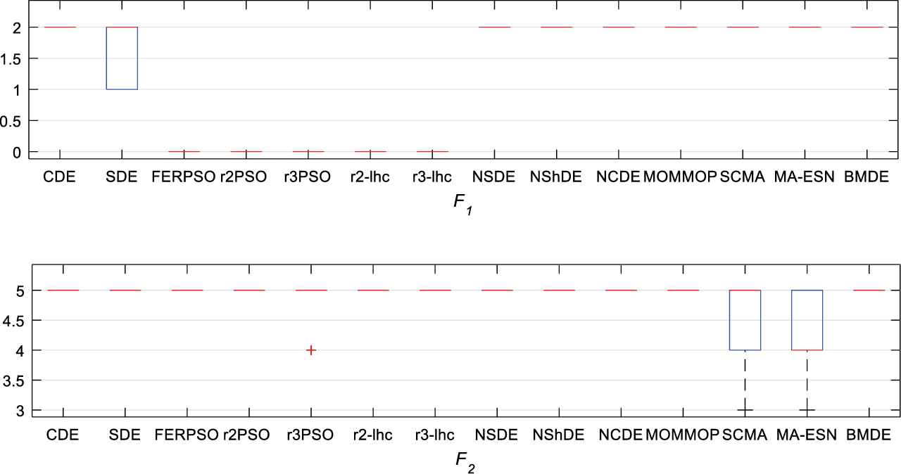
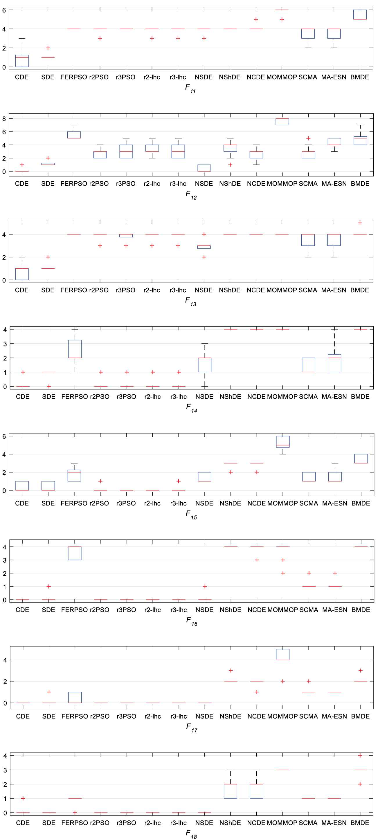
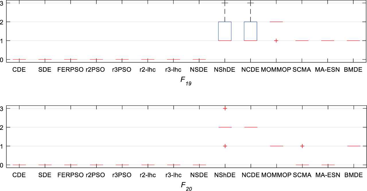
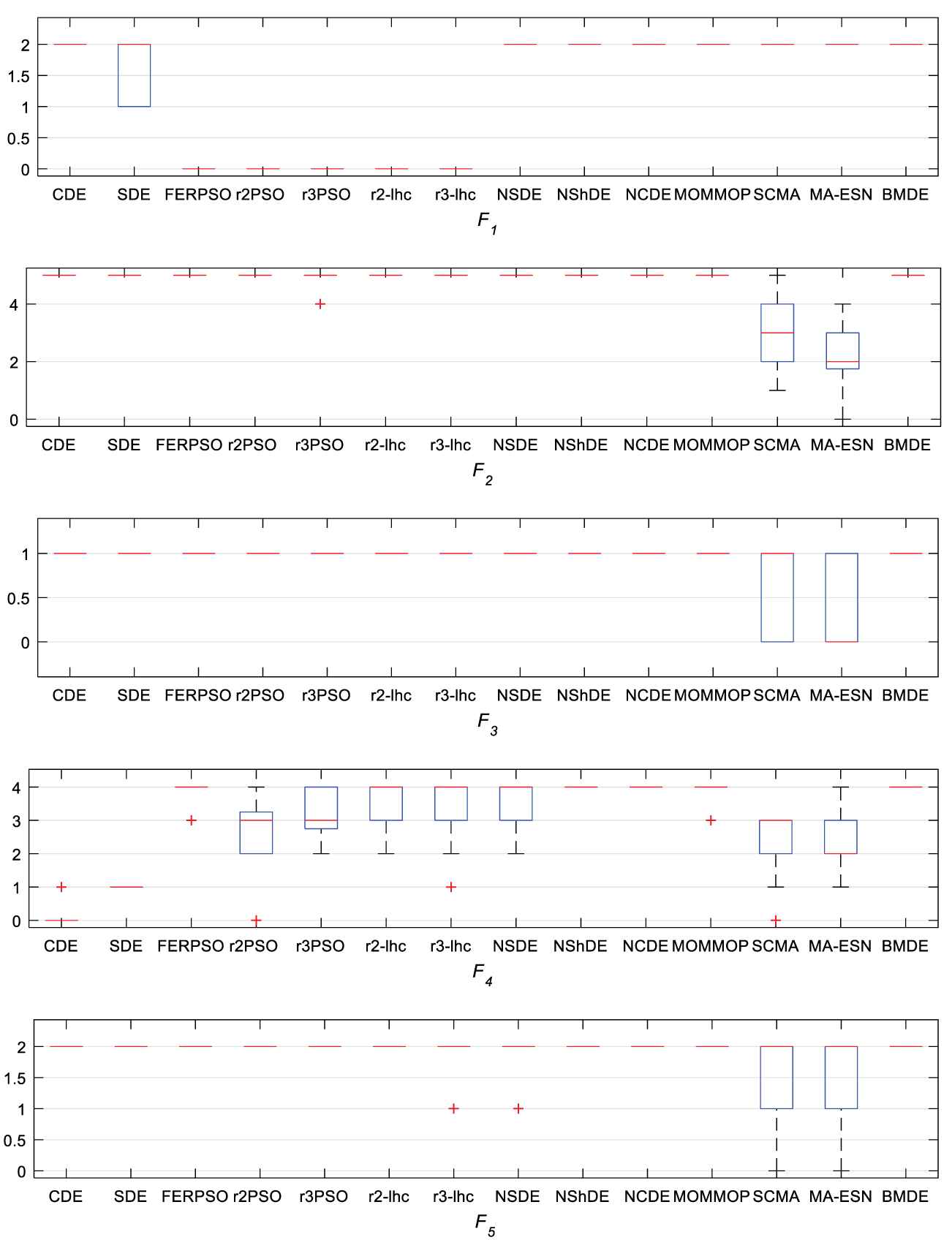
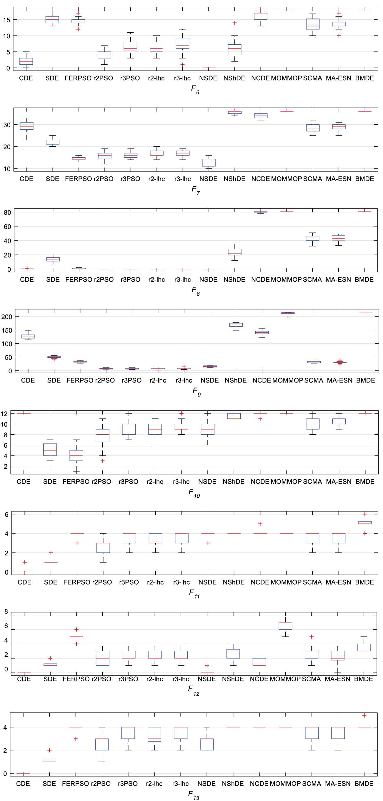
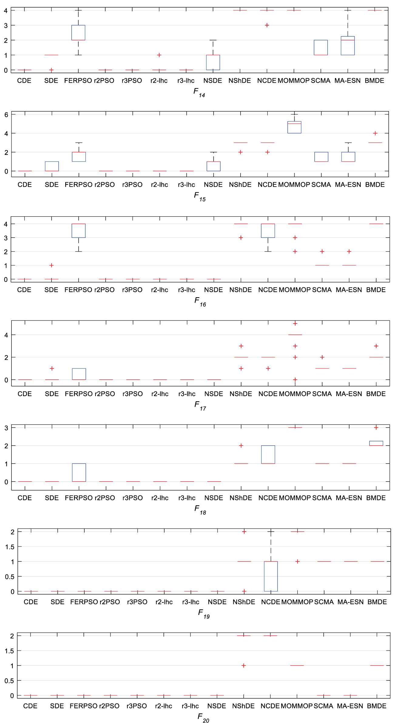
In order to intuitively display the number of global optimal solutions found by each algorithm, Figures 2–4 show the results of average number of peaks (ANP) obtained in 25 independent runs by each algorithm for function F₁–F₂₀ at ε = 1.0E−3, ε = 1.0E−4, and ε = 1.0E−5, respectively. ANP denotes the average number of peaks found by an algorithm over all runs. In addition, in order to make Figures 2–4 clearer, r2PSO-lhc, r3PSO-lhc, SCMA-ES are denoted as r2-lhc, r3-lhc, and SCMA for short, respectively.

Figure 2

Box-plot of ANP found by BMDE, CDE, SDE, FERPSO, r2PSO, r3PSO, r2PSO-lhc, r3PSO-lhc, NSDE, NShDE, NCDE, MOMMOP, SCMA-ES, and MA-ESN on F₁−F₂₀ at accuracy level ε = 1.0E−3. ANP, average number of peaks; BMDE, bi-population and multi-mutation differential evolution; NSDE, neighborhood-based SDE; CDE, crowding differential evolution; SDE, species differential evolution; FERPSO, fitness-Euclidean distance ration particle swarm optimization; PSO, particle swarm optimization; NShDE, neighborhood-based sharing DE; NCDE, neighborhood-based CDE; MOMMOP multiobjective optimization for MMOPs; SCMA-ES, self-adaptive niching CMA-ES; MA-ESN, matrix adaptation evolution strategy with dynamic niching.

Figure 3

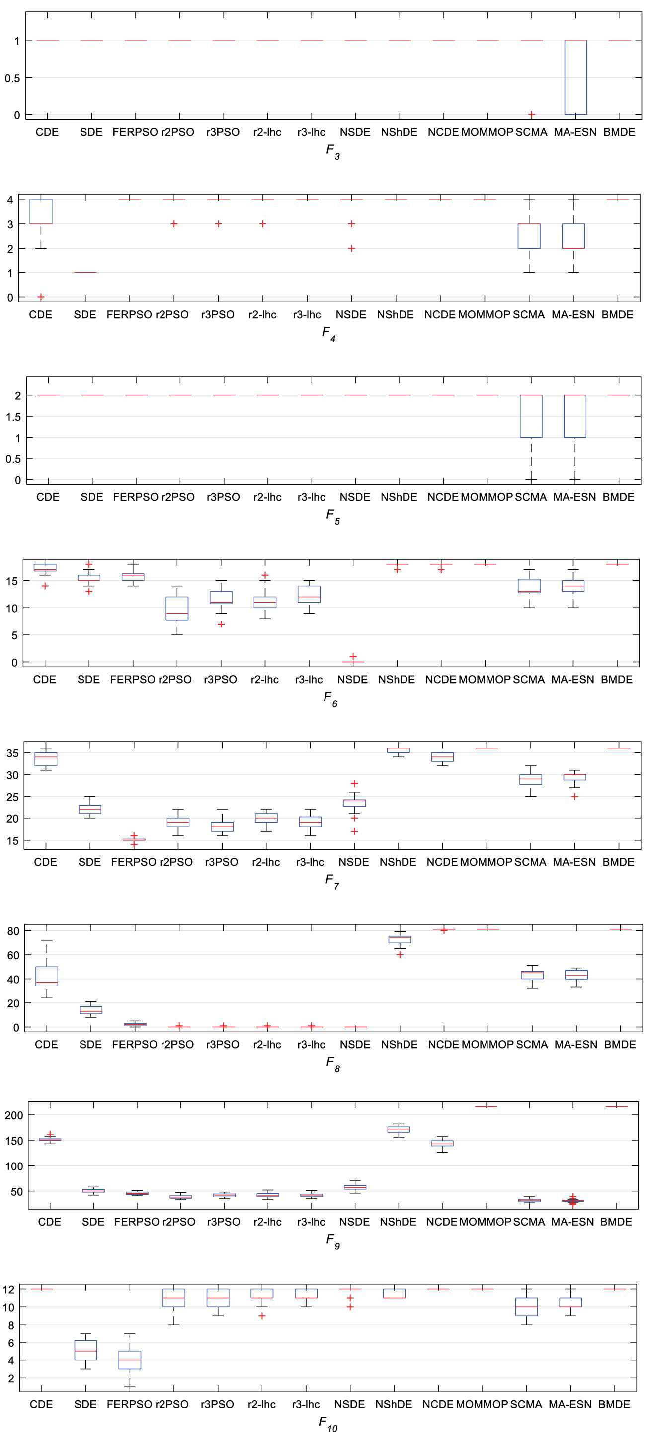
Box-plot of ANP found by BMDE, CDE, SDE, FERPSO, r2PSO, r3PSO, r2PSO-lhc, r3PSO-lhc, NSDE, NShDE, NCDE, MOMMOP, SCMA-ES, and MA-ESN on F₁−F₂₀ at accuracy level ε = 1.0E−4. ANP, average number of peaks; BMDE, bi-population and multi-mutation differential evolution; NSDE, neighborhood-based SDE; CDE, crowding differential evolution; SDE, species differential evolution; FERPSO, fitness-Euclidean distance ration particle swarm optimization; PSO, particle swarm optimization; NShDE, neighborhood-based sharing DE; NCDE, neighborhood-based CDE; MOMMOP multiobjective optimization for MMOPs; SCMA-ES, self-adaptive niching CMA-ES; MA-ESN, matrix adaptation evolution strategy with dynamic niching.

Figure 4

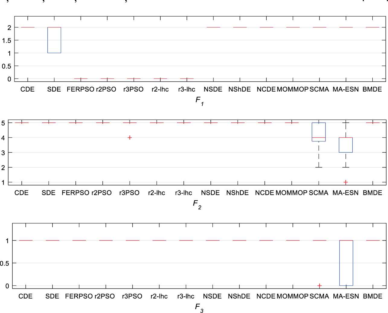
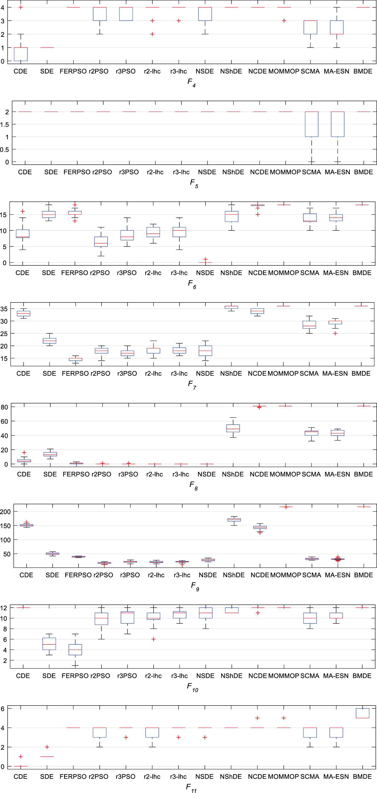
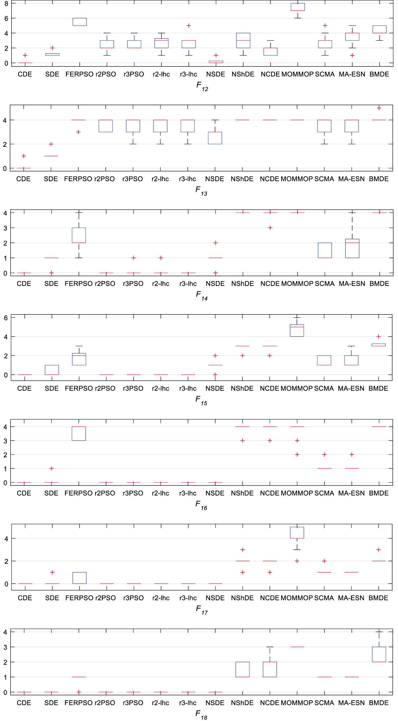
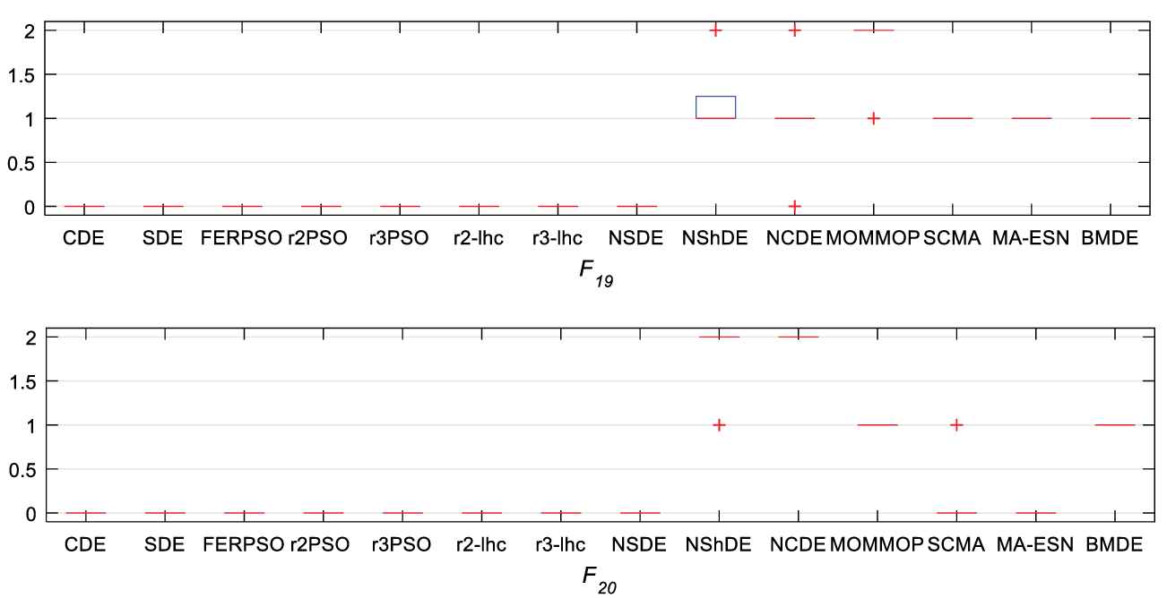
Box-plot of ANP found by BMDE, CDE, SDE, FERPSO, r2PSO, r3PSO, r2PSO-lhc, r3PSO-lhc, NSDE, NShDE, NCDE, MOMMOP, SCMA-ES, and MA-ESN on F₁−F₂₀ at accuracy level ε = 1.0E−5. ANP, average number of peaks; BMDE, bi-population and multi-mutation differential evolution; NSDE, neighborhood-based SDE; CDE, crowding differential evolution; SDE, species differential evolution; FERPSO, fitness-Euclidean distance ration particle swarm optimization; PSO, particle swarm optimization; NShDE, neighborhood-based sharing DE; NCDE, neighborhood-based CDE; MOMMOP multiobjective optimization for MMOPs; SCMA-ES, self-adaptive niching CMA-ES; MA-ESN, matrix adaptation evolution strategy with dynamic niching.