
Multi-Objective Particle Swarm Optimization Algorithm for the Minimum Constraint Removal Problem
- DOI
- 10.2991/ijcis.d.200310.005How to use a DOI?
- Keywords
- Minimum constraint removal; Minimum constraint set; Path planning; Multi-objective optimization; Multi-objective particle swarm optimization algorithm
- Abstract
This paper proposes a multi-objective approach for the minimum constraint removal (MCR) A problem. First, a multi-objective model for MCR path planning is constructed. This model takes into account factors such as the minimum constraint set, the route length, and the cost. A multi-objective particle swarm optimization (MOPSO) algorithm is then designed based on the fitness function of the multi-objective MCR problem, and an iteration formula based on the personal best (pbest) and global best (gbest) of the algorithm is constructed to update the particle velocity and position. Finally, compared with ant colony optimization (ACO) A and the crow search algorithm (CSA) A, the experimental results show that the MOPSO-based path planning algorithm can find a shorter path that traverses fewer obstacle areas and can thus perform MCR path planning more effectively.
- Copyright
- © 2020 The Authors. Published by Atlantis Press SARL.
- Open Access
- This is an open access article distributed under the CC BY-NC 4.0 license (http://creativecommons.org/licenses/by-nc/4.0/).
1. INTRODUCTION
Path planning is an important step for operating robots, robotic arms, and manipulators to accomplish predefined tasks; therefore, it is critical in robotic technologies [1]. The primary goal of path planning is to apply an analysis standard to find the shortest collision-free path for a robot from the initial state (including the position and posture) to the target state in an environment that contains obstacles [2]. Selecting the optimal path from the start position to the target position is the key issue in the early stage of robot path planning. To address this issue, most studies have focused on avoiding obstacles and have used global or local optimization to find the shortest obstacle-free path [3].
Not all robotic operational environments are obstacle free [4]. However, not all obstacles must be avoided. For example, in indoor navigation, the obstacle may be a closed door that a robot can open. In autonomous outdoor navigation, the obstacle may be an area of rough but not insurmountable terrain that a robot can pass through. However, in these situations, traversing the obstacle may be costly and risky. These two practical problems have sparked novel ideas in robot path planning research. In 2012, Hauser proposed a new path planning problem, which is called the minimum constraint removal (MCR) problem [5]. The goal is to find the minimum number of geometrical constraints that should be removed to connect the start state to the target state via a free path. This requires the removal of the minimum number of constraints (obstacles) to create an obstacle-free path in the environment. MCR path planning takes into account the possibility that the robot may not be able to find an obstacle-free path and attempts to find a path for the robot with minimal constraints. In this context, constraints are obstacles or areas of obstacles along the route. The significance of MCR path planning is that even if the robot must travel across constraints along a path, an effort should be made to ensure that the path traverses the minimum number of constraints. Once such a path has been found, whether by clearing the obstacles in the path or crossing areas of obstacles, higher efficiency will be achieved [6].
The MCR problem has recently become a popular research topic in the area of path planning. The MCR problem was initially proposed in 2012 by Hauser [5], who employed a method of reduction from the minimum set cover to prove that the discrete MCR problem is non-deterministic-polynomial-hard (NP-hard) A. He provided numerous new discrete theoretical MCR results and employed two search algorithms that have excellent practical performance, the exact search algorithm and the greedy search algorithm, to solve the discrete MCR problem. Hauser also demonstrated three use cases: the generation of a failure reason that is understandable by humans, motion planning in an uncertain environment, and the selection of a movable obstacle in a complicated environment [7]. The exact search algorithm and the greedy search algorithm take the minimum-obstacle constraint set as the target and pursue the optimal solution instead of satisfying a solution that meets the requirements at that time.
Erickson and LaValle used the reduction of the maximum satisfiability problem for the binary Horn clause to prove that the discrete MCR problem is NP-hard [8], but the Horn clause satisfiability method had very strict restrictions on the diagrams and obstacles obtained by transformation. Cohen focused on robotic arm path planning, constructed a discrete MCR model, and demonstrated that the discrete MCR problem is also NP-hard; he then employed a breadth-first algorithm that was based on graph-cut theory to find the path with minimum constraints to improve the robotic arm's operational efficiency [9], but this algorithm also aimed for the minimum-obstacle constraint set. Krontiris and Shome also leveraged graph theory to solve the MCR problem in robot path planning; the start and target positions were set to the graph's source point and sink point, respectively, and the maximum flow and minimum cut methods were employed to complete the MCR path planning [10], but the effect of their method was not very satisfactory. Sharon employed a multi-agent system intelligent algorithm to solve the multi-robot MCR path search problem, which took into account conflicts between individual robots and used a coordinated multi-agent mechanism to determine the path with minimum constraints [11]. However, their method relied on the learning ability of agents. Gorbenko and Popov investigated the discrete MCR problem in motion planning that could be used for path planning with an explanation for failure and an efficient approach to solving the problem. In particular, they investigated an explicit reduction of a decision version of the problem to a satisfiability problem [12], but the process for proving was very complicated. Krontiris and Bekris used the graph method to solve the rearrangement problem; set the starting position and the target position as the source point and the junction point of the graph, respectively; and proposed an approximate but significantly accelerated monotonic rearrangement method. This method defined the dependency graph between objects and allowed each object to reach its target by finding the MCR path [13]. Krontiris and Bekris also proposed a bounded length method to find a path of a certain length that could balance between minimum constraints, cost calculation, and route length [14,15], but they considered only cost and path length in the method. Bandyapadhyay proposed improved approximation bounds that gave an
Our research team believes that once discrete MCR problems have been confirmed to be NP-hard, the primary focus should shift to the use of various intelligent heuristic algorithms to solve these problems. Therefore, a highly effective approximate solution method should be developed. In our previous study, an ant colony optimization (ACO) algorithm was introduced to solve the MCR problem in motion planning; the algorithm achieved the desired goal because the solution quality and convergence speed were superior to those of the accurate search and greedy algorithms. For details, please refer to our previous research findings [17,18]. In the past, we worked from only a single target.
Current research on solving the MCR problem has made substantial progress; however, the main idea is to convert continuous MCR problems into discrete MCR problems and then use various methods to solve the discrete problems. To date, the researchers have used the greedy search algorithm, the exact search algorithm, and ACO to solve the MCR problem. However, these methods fail to achieve satisfactory results due to inherent defects and isolate the complex relationships among objects, robots, and obstacles in the process of solving MCR problems. For example, factors such as route length and cost are seldom addressed. However, in complex environments, the MCR problem is dynamic and multi-objective in nature; factors such as the minimum constraint set, route length, and cost should be considered. Therefore, this paper proposes a multi-objective approach for the MCR path planning problem.
2. PRELIMINARIES
2.1. Mathematical Model for MCR Path Planning
To facilitate this research, the MCR problem in robot path planning is described first. A typical MCR path planning scenario is shown in Figure 1.
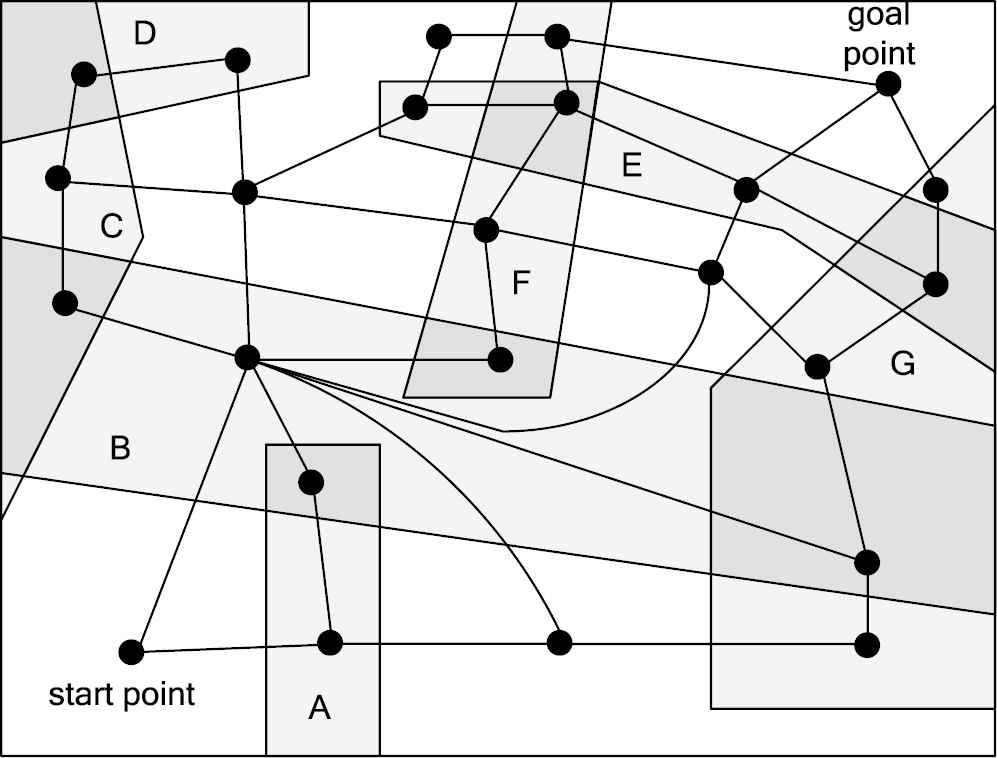
A typical scenario of MCR path planning.
In Figure 1, the robot starts at the start point in the lower-left corner and ultimately reaches the goal point in the top-right corner. This scenario contains seven obstacle areas, which are denoted as obstacles A, B, C, D, E, F, and G. The goal of MCR path planning is to plan a path from the start point to the goal point that traverses the minimum number of obstacles.
In Figure 1, the black dots represent nodes along each path where the robot can stay. All the nodes constitute a node network (Figure 2). In Figure 2, some of the nodes are labeled with obstacle names; for example, the label “B, G” means that the node is covered simultaneously by obstacles B and G. Some of the nodes are not labeled with obstacle names because they are not covered simultaneously by obstacles.
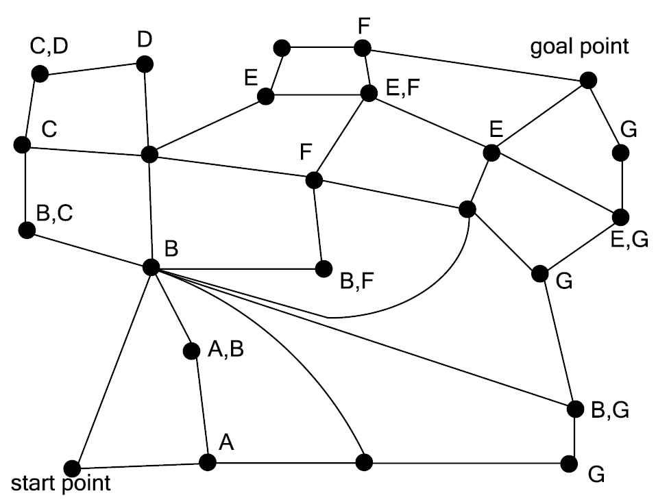
Node network for MCR path planning.
If the robot follows a path that contains node B, G, it must pass at least two obstacle areas, B and G. In this way, the MCR path planning problem is transformed into a problem to find a path that passes a series of nodes and is covered by the minimum number of obstacles in the node network (Figure 2).
Next, the MCR path planning problem is described via a mathematical model. The mathematical model for the continuous MCR problem is defined as follows:
Input: It is assumed that all the nodes in the node network constitute a set, which is denoted as
Definition 1:
A cover function
Definition 2:
For a label subset
Output: The MCR set
The discrete MCR problem is elaborated further via graph theory. The node set and the path that connects these nodes constitute a graph, which is represented as
In addition, this graph is associated with the cover function
The discrete MCR problem is defined as follows:
Input: The input includes the graph
Output:
Furthermore, if there is a label subset
2.2. Multi-Objective Optimization
A 3-tuple
Feasible solution—definition 1:
Feasible solution set—definition 2: a set of all feasible solutions
Pareto dominated—definition 3: for decision vectors
Pareto optimal solution—definition 4: if a feasible solution
Pareto optimal solution set—definition 5: the Pareto optimal solution set is the set of all Pareto optimal solutions.
The goal of multi-objective optimization is to achieve a uniform distribution of the solution set and a fast approximation to the actual Pareto frontier. Based on this goal, researchers have proposed numerous effective multi-objective evolutionary algorithms. The research on evolutionary multi-objective optimization algorithms can be divided into three phases. In phase 1, Pareto dominance was employed to design a simple fitness function; typical algorithms include the multi-objective genetic algorithm (MOGA) A by Fonseca and Fleming, the niched Pareto genetic algorithm (NPGA) A by Horn and Nafpliotis, and the non-dominated sorting genetic algorithm (NSGA) A by Srinivas and Deb [20]. In phase 2, an elitist group was employed to maintain the current Pareto optimal solution's distribution properties; typical algorithms include the Pareto archived evolutionary strategy (PAES) A by Knowles et al., the strength Pareto evolutionary algorithm (SPEA) A and SPEA2 by Zitzler and Thiele et al. [21], and the improved NSGA A (NSGA-II), which is based on an elitist strategy, by Deb and Pratap et al. [22]. In phase 3, hybrid algorithms were developed from combinations of the multi-objective evolutionary algorithm and other emerging intelligent algorithms, such as the immune multi-objective optimization algorithm (IMOA) A [23] and multi-objective particle swarm optimization (MOPSO) A [24].
3. MULTI-OBJECTIVE MODEL FOR MCR PATH PLANNING
In the real world, the MCR problem has multiple objectives, and the goals are complex, dynamic, and influenced by many factors. The robot will face a complex and dynamic MCR path. Based on these characteristics, the real-world multiple-objective MCR problem is abstracted into a mathematical model to create a multi-objective model for MCR path planning.
Because several influencing factors of the MCR path planning problem are correlated and affect each other, they should be taken into account as a whole. Further, the actual conditions should be satisfied. The following three factors are taken into account: the number of minimum obstacles in the constraint set
Assume that an obstacle in the real environment is denoted as
Assume that any robot
Definition 1 (Necessary condition):
The minimum constraint set
Definition 2:
The total cost to remove the obstacles in the minimum constraint set
Definition 3:
The route length calculation is as follows:
The multi-objective model for the MCR path planning problem is described as follows. When the precondition of the minimum constraint set
4. MCR PATH PLANNING BASED ON MULTI-OBJECTIVE PARTICLE SWARM OPTIMIZATION ALGORITHM
In the conventional robot path planning problem, several intelligent optimization algorithms are employed for path search and optimization. After the MCR problem was developed, intelligent algorithms, such as the greedy algorithm and the ACO algorithm, were applied to MCR path planning. The particle swarm algorithm is also a typical intelligent optimization algorithm. This paper applies the particle swarm optimization (PSO) A algorithm to multi-objective MCR path planning and designs a MOPSO algorithm according to the characteristics of the MCR multi-objective path planning problem.
When the PSO algorithm is used to solve a multi-objective optimization problem, the key is to select the personal best (pbest) and global best (gbest) of the PSO algorithm. Three general goals of multi-objective optimization should be satisfied [25]: to obtain the maximum number of Pareto solutions, to ensure that the obtained Pareto solution set is as close to the actual Pareto frontier as possible, and to maximize the Pareto solution's distribution range. It is fairly easy to determine the individual leader in a single objective problem because there is only one gbest at each moment. However, in multi-objective optimization, because the non-dominated solution is not unique, each particle should identify a gbest in a leader set to update its own position; the swarm should take into account not only the optimization level of the “solution” but also the distribution of the Pareto frontier. The diversity of the swarm should also be maintained to avoid local optima.
Assuming that a particle swarm contains
In this paper, path planning involves more than the position. Therefore, a fitness function is used for the evaluation. The state of
For the multi-objective MCR path planning problem, particles are randomly generated at the start point
Based on this analysis and the aforementioned idea of a MOPSO-based solution to the MCR problem, a simple and highly effective multi-objective particle swarm algorithm is proposed to address the MCR problem. The procedure of the algorithm is as follows (Figure 3):
The procedure of the MCR path planning algorithm.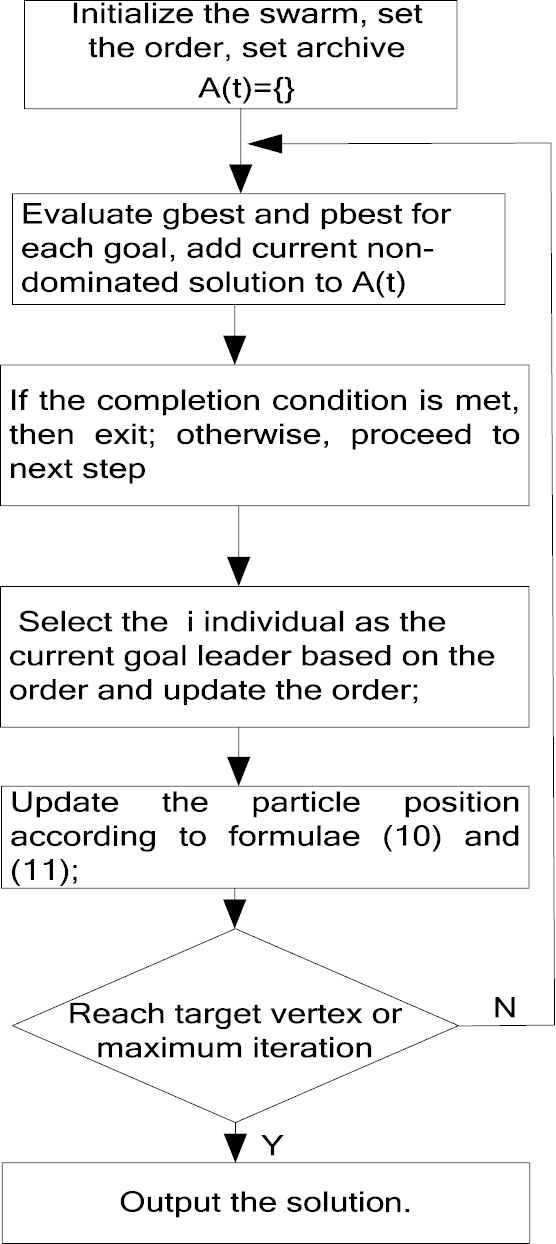
First, the algorithm randomly generates an initialized swarm and an empty archive and sets an order. The gbest and historical pbest for each objective function are then evaluated, the non-dominated solution for the current generation of individuals is archived, and the individuals that are dominated by the current solution are deleted from the original archive. If the storage exceeds the threshold, then some elements are deleted based on certain rules. In step 4, the goal leader is identified based on the order; the particle position is then updated based on the goal leader, and the order is modified. This process is repeated until the constraint conditions are satisfied.
5. EXPERIMENT RESULT AND ANALYSIS
To verify the effectiveness of the proposed MOPSO method, the following experiment is performed.
The test scenario is assumed to be a 10*10 grid area. Therefore, the entire test scenario contains 100 grid sub-blocks; the obstacle area is randomly generated and contains at least one grid. The four vertexes of a grid are nodes, which are positions where the robot can stay. Figure 4 shows the entire test scenario.
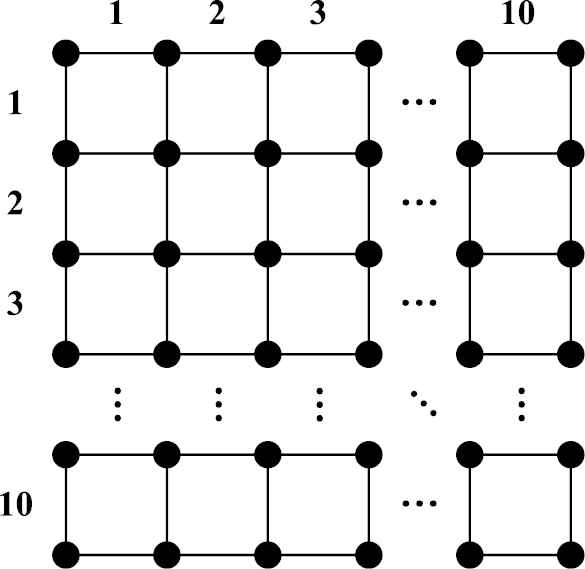
Diagram of the test scenario.
In this test, the maximum iteration of the MOPSO will not exceed 1000. In addition, the ACO algorithm in reference [18] and the crow search algorithm (CSA) in reference [26] are compared with the proposed algorithm. Two sets of test data with the following detailed settings are configured:
V = 25, E = 80, S = 10, 20;
V = 441, E = 1680, S = 10, 20.
The three algorithms are executed separately, and the results are shown in Tables 1 and 2 and Figures 5 and 6. In the results, K denotes the number of removable obstacles, Cost denotes the cost to remove obstacles, R(L) denotes the route length, and Cover denotes the obstacles to be removed. The following formula is defined for the test:
| Found Solution | R(L) | Cost | K [Cover] | ||
|---|---|---|---|---|---|
| V = 25 | ACO | True | 24 | 13 | 2 [‘O2’, ‘O3’] |
| E = 80 | CSA | True | 24 | 13 | 2 [‘O2’, ‘O3’] |
| S = 10 | MOPSO | True | 24 | 13 | 2 [‘O2’, ‘O3’] |
| V = 25 | ACO | True | 38 | 256 | 5 [‘O2’, ‘O3’, ‘O8’, ‘O9’,‘10’] |
| E = 80 | CSA | True | 28 | 156 | 4 [‘O2’, ‘O3’, ‘O8’, ‘O9’] |
| S = 20 | MOPSO | True | 28 | 156 | 4 [‘O2’, ‘O3’, ‘O8’, ‘O9’] |
The best path comparison of the two algorithms in test data 1.
| Found Solution | R(L) | Cost | K [Cover] | ||
|---|---|---|---|---|---|
| V = 441 | ACO | True | 413 | 42 | 3 [‘O1’, ‘O4’, ‘O5’] |
| E = 1680 | CSA | True | 413 | 42 | 3 [‘O1’, ‘O4’, ‘O5’] |
| S = 10 | MOPSO | True | 413 | 42 | 3 [‘O1’, ‘O4’, ‘O5’] |
| V = 441 | ACO | True | 441 | 223 | 5 [‘O1’, ‘O10’, ‘O4’, ‘O5’, ‘O9’] |
| E = 1680 | CSA | True | 441 | 223 | 5 [‘O1’, ‘O10’, ‘O4’, ‘O5’, ‘O9’] |
| S = 20 | MOPSO | True | 421 | 207 | 5 [‘O1’, ‘O10’, ‘O5’, ‘O9’] |
The best path comparison of the two algorithms in test data 2.
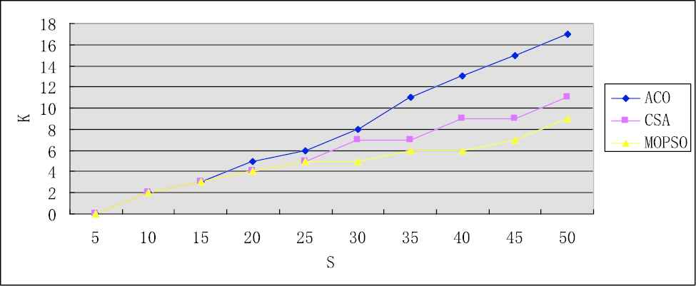
Comparison of the number of removable obstacles (V = 25, E = 80).
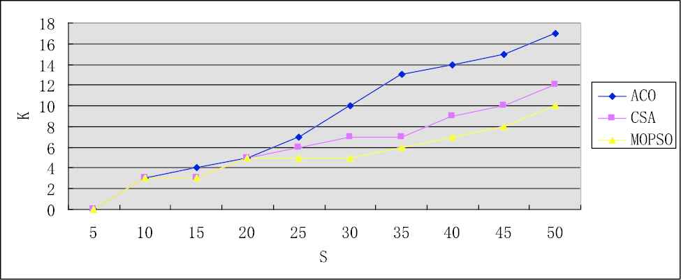
Comparison of the number of removable obstacles (V = 441, E = 1680).
SPSS 19.0 statistical analysis software was used to process the data. We ran 50 experiments; the Wilcoxon test was used to compare the counting data. P < 0.05 was considered statistically significant. The statistical results show the following. In test data 1, compared with the MOPSO algorithm, the ACO and CSA algorithms had longer path lengths, higher costs, and more obstacles, but there was no significant difference between the MOPSO and CSA algorithms (P > 0.05) or between the MOPSO and ACO algorithms (P > 0.05). In test data 2, compared with the MOPSO algorithm, the ACO and CSA algorithms had longer path lengths, higher costs, and more obstacles, and there was a significant difference between the MOPSO and CSA algorithms (P < 0.05) and between the MOPSO and ACO algorithms (P < 0.05).
In Figures 5 and 6, S denotes the number of obstacles, and K denotes the number of removable obstacles. Tables 1 and 2 show that path planning using the MOPSO algorithm proposed in this paper can find a shorter optimal path at a lower cost than using the ACO and CSA algorithms. Moreover, with an increase in the number of obstacles, the advantage of path planning using the MOPSO algorithm increases.
Figures 5 and 6 also show that with an increase in the number of obstacles in the scenario, all the optimal paths that were identified by the three algorithms contain obstacles. The paths that were identified by the path planning algorithms that used the ACO and CSA algorithms contain significantly more obstacles, and this trend is magnified as the number of obstacles increases. A comparison of the results in Tables 1 and 2 and Figures 5 and 6 shows that because of the superiority of the MCR planning result, the proposed algorithm is superior.
Figures 7 and 8 show the Pareto solution set distribution of the MOPSO algorithm.
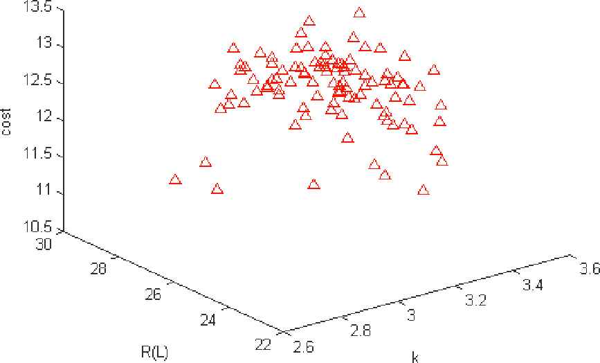
Pareto solution set distribution of the MOPSO algorithm (V = 441, E = 1680, S = 10, 500 iterations).
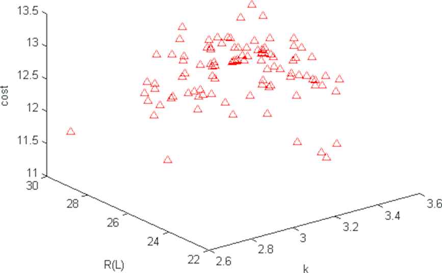
Pareto solution set distribution of the MOPSO algorithm (V = 441, E = 1680, S = 10, 1000 iterations).
Figures 7 and 8 show that the MOPSO algorithm has a wide search space and a large number of well-distributed solutions. The Pareto solution set space distributions in Figures 7 and 8 show relationships between three goal vectors: the shortest route length
6. CONCLUSIONS
This paper used the MOPSO algorithm for multi-objective MCR path planning. First, a multi-objective model for MCR path planning was constructed. A MOPSO algorithm was then designed based on the fitness function of the multi-objective MCR problem, and an iteration formula based on pbest and gbest was constructed to update the particle velocity and position. Finally, a comparison with the ACO and CSA algorithms showed that in scenarios with an identical number of obstacles, the MOPSO path planning algorithm can obtain a shorter best path that traverses fewer obstacle areas, which is better for solving the MCR path planning problem, and provide a global optimization plan for MCR path planning that satisfies multiple design goals. A single execution of the algorithm obtains multiple Pareto optimal solutions, which provides a reference and can be applied to actual cases.
The MCR problem in complex environments is a new MCR research problem. The contradictions between the targets and the dynamic changes between the obstacles and the robot are research challenges for the MCR problem in complex environments.
CONFLICT OF INTEREST
Authors have no conflict of interest to declare.
AUTHORS' CONTRIBUTIONS
Bo Xu and Feng Zhou conceived and designed the study, performed the experiments and wrote the paper. Antonio Marcel Gates reviewed and edited the manuscript. All authors read and approved the manuscript.
ACKNOWLEDGEMENTS
This work was supported by the National Natural Science Foundation of China (11901113), Natural Science Foundation of Guangdong Province (2018A030307032), and the Guangzhou Science and Technology Plan Project, China (201904010225). The authors thank all the reviewers and editors for their valuable comments and work.
Appendix A
| Minimum constraint removal | MCR |
| Ant colony optimization | ACO |
| Crow search algorithm | CSA |
| Particle swarm algorithm | PSO |
| Non-deterministic-polynomial-hard | NP-hard |
| Multi-objective genetic algorithm | MOGA |
| Niched Pareto genetic algorithm | NPGA |
| Non-dominated sorting genetic algorithm | NSGA |
| Pareto archived evolutionary strategy | PAES |
| Strength Pareto evolutionary algorithm | SPEA |
| Immune multi-objective optimization algorithm | IMOA |
| Multi-objective particle swarm algorithm | MOPSO |
REFERENCES
Cite this article
TY  - JOUR
AU  - Bo Xu
AU  - Feng Zhou
AU  - Antonio Marcel Gates
PY  - 2020
DA  - 2020/03/16
TI  - Multi-Objective Particle Swarm Optimization Algorithm for the Minimum Constraint Removal Problem
JO  - International Journal of Computational Intelligence Systems
SP  - 291
EP  - 299
VL  - 13
IS  - 1
SN  - 1875-6883
UR  - https://doi.org/10.2991/ijcis.d.200310.005
DO  - 10.2991/ijcis.d.200310.005
ID  - Xu2020
ER  -