
Optimal Core Operation in Supply Chain Finance Ecosystem by Integrating the Fuzzy Algorithm and Hierarchical Framework
- DOI
- 10.2991/ijcis.d.200226.001How to use a DOI?
- Keywords
- Supply chain finance (SCF); Fuzzy theory; Analytic hierarchy process (AHP); Smartphone industry supply chain; Core operation (CO)
- Abstract
Supply chain finance (SCF), which has the key concept of the delivery of credit, is a new type of financial service that can enhance the financial efficiency of a supply chain. Using the transaction records from the core operations (CO) of the members, financers can provide a higher level of cash flow to the ecosystem. Moreover, financial sectors can upgrade their operations through SCF activities. However, while SCF services can help financial sectors improve their operations, there are many risks implied in SCF activities from CO to relative members. Therefore, this paper presents a novel model that applies a combination of triangular fuzzy numbers and the analytic hierarchy process (AHP) to the decision-making process to evaluate the decision behaviors regarding the preference the CO in the smartphone industry supply chain for financers in the SCF service. Academically, the FAHP-based decision-making framework can provide the decision makers and administrators of financial institutions with valuable guidance for measuring the optimal CO of the smartphone industry in the SCF ecosystem. Commercially, the proposed model could provide administrators with a useful tool to assess the optimal CO of the smartphone industry within the SCF ecosystem for financers.
- Copyright
- © 2020 The Authors. Published by Atlantis Press SARL.
- Open Access
- This is an open access article distributed under the CC BY-NC 4.0 license (http://creativecommons.org/licenses/by-nc/4.0/).
1. INTRODUCTION
The development of the globalized economy in recent years has led to intense market competitions; hence, many industries have implemented supply chain management (SCM). SCM has attracted wide attention, as the opportunities of integrated supply chain can reduce the propagation of unexpected events throughout the network, decisively influence the profitability of all supply chain members, and co-ordinate all input/output flows (materials, information, and finances) [1,2]. In addition to manufacturing, logistics, and marketing activities, SCM systems rely on financial processes to coordinate the flow of goods, services, and money between the separate stages of a supply chain [3]. The financial processes that can be seen are important to all industries when implementing supply chain activities; therefore, finance organizations are willing to provide small and medium-sized enterprises (SMEs) with working capital to them to expand their market share. This concept is the basis of supply chain finance (SCF), as it can improve the efficiency of financial flows (FFs) in a supply chain.
The concept of SCF was proposed in 2006 [4]. Pfohl and Gomm [5] proposed the definition of SCF as inter-company optimization of financing, as well as the integration of financing processes with customers, suppliers, and service providers, in order to increase the value of all participating companies. Randal and Farris [6] found that SCF can strengthen a supply chain through the collaborative management of cash-to-cash cycles and sharing the weighted average cost of capital. SCF can create financial win-win situations for buyers, sellers, and financial intermediaries [7]. From the bankers’ perspectives, the main feature of SCF is to identify the core operation (CO) in the supply chain, and improve its financial constitution, which extends the good credit of the CO to the upstream and downstream enterprises, and improves lending without taking on unacceptable risks [8,9]. The three flows of the traditional SCM system (financial, goods, and information) are shown in Figure 1, while Figure 2 shows the SCF ecosystem. For example, if the CO is a manufacturer, supply chain members (upstream/downstream) can extend credit by the CO to enhance their working capital efficiency, which can solve the problem faced by most SMEs, meaning they have low credit to receive loan funds. Therefore, the CO in a SCF ecosystem is a critical role for a bank.
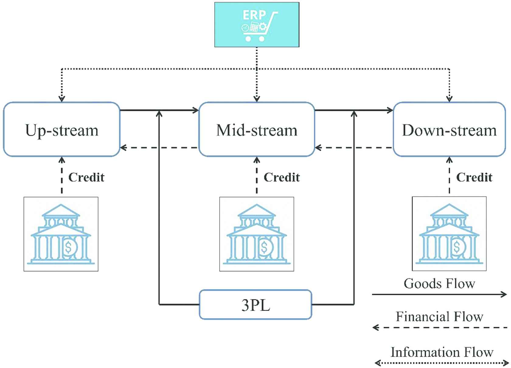
The three flows of the traditional SCM system.
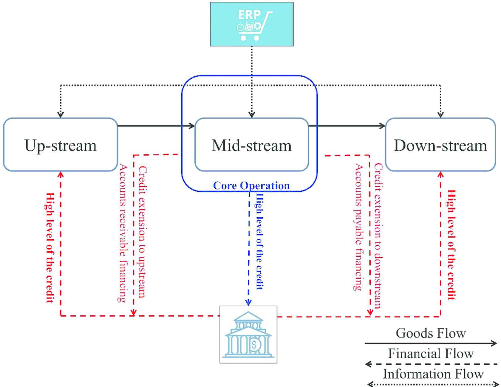
The ecosystem of SCF.
In this economic environment it is very difficult to access funds through traditional channels, and with banks tending to lend less, corporations are finding alternative ways to source funding. Lack of access to required financing has strained many buyer/supplier relationships [7], and the SCF ecosystem may solve this problem for supply chain members. The SCF ecosystem is a new financial service that makes supply chain more efficient by providing SMEs with a lower cost of credit. Some studies have identified the benefits of banks providing SCF services in a supply chain, which are enhanced profitability, stronger collaborative relationships with clients, increased reach and profile of trade, treasury organizations, and expanded lending banking services [10,11].
SCF inherits numerous risks through the CO to the upstream and downstream members in a supply chain ecosystem. These risks include supply chain systematic risk, transaction risk, and bankruptcy risk, and so on ([12,13], Gao et al., 2018). Many previous studies have examined the risks in various industries; however, evidence on the evaluation of the optimal CO regarding SCF issues for financers is few. Thus, it is important to evaluate the optimal CO when a financer provides SCF services.
To date, no research has developed a comprehensive model for CO evaluation in SCF ecosystems via fuzzy theory and decision science; hence, the purpose of this study is to present a novel model based on the combination of fuzzy logic and the analytic hierarchy process (AHP) using a case study of the smartphone industry supply chain, in order to assess which operation provides the optimal CO for financers. As evaluating the CO in a supply chain is important for SCF [14], determining the optimal CO is a decision science problem and the ideal model requires suitable criteria and strict screening [15]. Tsai et al. [16] indicated that the AHP method is a decision science method that can evaluate and prioritize the weights of each criteria and alternatives. However, AHP cannot adequately resolve the inherent uncertainties and imprecisions associated with mapping the decision maker's perceptions into exact numbers [16]. In addition, few literatures regarding SCF and the smartphone industry have applied the fuzzy method and AHP to evaluate the optimal CO of the smartphone supply chain for the financial sector. The smartphone industry is chosen for this case study due to its complex supply chain, keen competition, unpredictable raw material values, and high purchasing costs [17], which affect the operational efficiency of their supply chain significantly. Therefore, determining the CO in this industry's SCF would allow the SMEs of the supply chain members to increase their financial efficiency through lower borrowing costs, thus solving the loan barrier via CO. It can be difficult to identify the CO in a smartphone industry supply chain, as the CO is often not readily apparent. As there are different sized firms in many parts of the supply chain, the CO cannot be identified without comprehensive analysis and there is no easy rule to identify it, as it can be in any part of the supply chain; thus, a comprehensive model is needed to identify the CO.
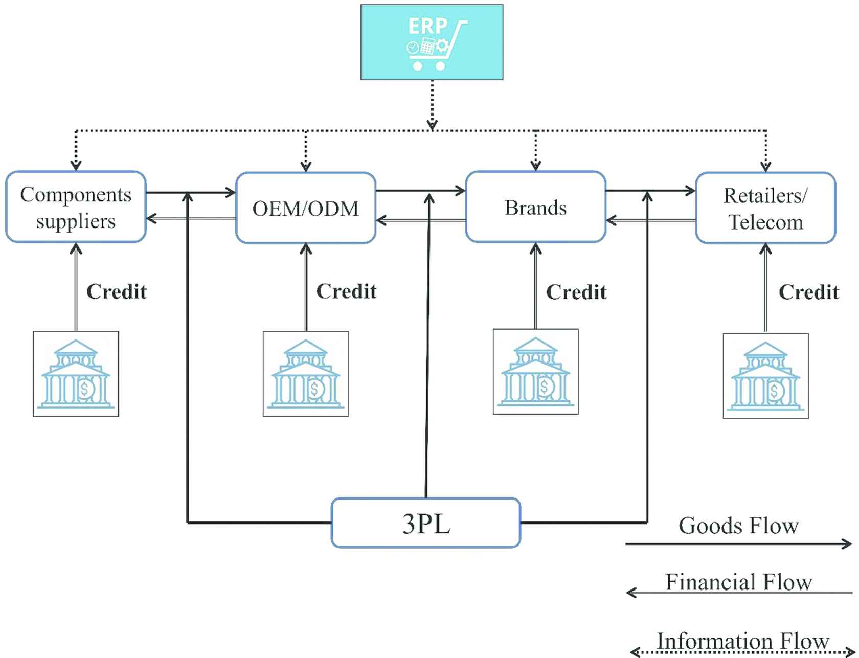
The main process of the smartphone industry supply chain can be divided into (1) components supplier, (2) original equipment manufacturer/original design manufacturer (OEM/ODM), (3) brands, and (4) retailer/telecom [18,19], as shown in Figure 3.
The Smartphone industry supply chain process.
While some papers regarding SCF cover concentrated coordination, working capital, and optimal FF [5,20,21], they have not solved the crucial problem of identifying the core of SCF ecosystem, that is, what exactly is the CO of a supply chain. Determining what constitutes the CO of the smartphone industry supply chain is critical to improving the efficiency of credit. The common financial model of a supply chain has one large company surrounded by SMEs. Currently, financial institutions lend separately to companies in every step of the supply chain; for example, manufacturers have a slightly different method of obtaining credit. Specifically, it sends its product to the retailer, and receives an accounts payable promissory note, which is then sent to the financial institution to allow it to obtain credit to pay the manufacturer for the product. Finding the optimal CO allows for a far more efficient model, where every member of the supply chain can use the upstream and/or downstream transaction records to obtain credit from the manufacturer. As finding the CO in a supply chain ecosystem is important [14], the evaluation of the optimal solution is a multi-criteria problem and the ideal model requires suitable criteria and strict screening [15]. Few literatures regarding SCF and the smartphone industry have used the multi-criteria decision-making (MCDM) concept to evaluate the optimal CO of the smartphone supply chain for a bank.
Optimal alternative evaluation is an MCDM problem that employs the AHP method to prioritize the weights of each criteria and alternatives [16], thus, many studies have applied AHP to construct a hierarchy architecture able to structure MCDM topics [22–25]. Even though AHP is commonly used, this algorithm cannot adequately resolve the inherent uncertainties and imprecisions associated with mapping decision maker's perceptions into exact numbers [16]. Hence, numerous previous studies have combined the fuzzy set theory with AHP to solve uncertain issues [26–31]. Zhü [32] proposed that fuzzy AHP (FAHP) cannot resolve uncertain questions. However, Fedrizzi and Krejčí [33] indicated that Zhü [32] had no reliable evidence for this result; thus, FAHP remains an interesting research topic with challenging development possibilities both in theory and application. Evaluating and prioritizing multiple criteria and their alternatives is complicated and challenging. Ayhan [34] indicated that uncertain and vague expert opinions result in more complications, meaning it is quite challenging for human beings to quantitatively predict given problems, as compared to qualitative prediction [34,35]. In such cases, the FAHP framework assists to translate the qualitative expressions of human beings into meaningful numeric predictions [36]. The FAHP methodology has been applied to rate human-opinion based optimal alternatives selection problems [35]. Therefore, this study develops a FAHP-based evaluation framework for fuzzy prioritization, where expert comparison judgments are represented by fuzzy triangular numbers. FAHP is adopted as the evaluation method, and its effectiveness is illustrated by numerical examples. In addition to literature review and surveying experts in the financial field, this study utilizes the modified Delphi method and FAHP to construct an evaluation process able to estimate the optimal CO of the smartphone industry supply chain in Taiwan for financers. Financers denote the financial sectors, financial institutions, funds, banks, and so on, which are to provide the SCF service in a supply chain. For example, a bank provides the SCF service for smartphone industry supply chain, and the members of SMEs in the smartphone industry supply chain are then able to improve the loan level by the CO with the bank.
Therefore, this study combines fuzzy theory and AHP to evaluate the synthetic utility values of the criteria and sub-criteria of the supply chain of the smartphone industry for the financial sector providing SCF services, and then assigns a suitable relative weight to each criterion within the fuzzy hierarchical model to rank the optimal CO. Academically, the FAHP-based decision-making framework can provide decision makers or administrators with valuable guidance for measuring the optimal CO of the smartphone industry in the SCF ecosystem. Commercially, the proposed model can provide administrators with a useful tool to assess the optimal CO of the smartphone industry within the SCF ecosystem for financers.
2. METHODOLOGY
The modified Delphi method is applied to collect expert opinions, identify the determinants of the evaluation model, and calculate the weighted criteria and ranking using FAHP. The Delphi method, AHP method, and FAHP method are described, as follows.
2.1. Delphi Method
This study applies the Delphi method to determine the evaluation sub-criteria. Using the Delphi method and expert interviews, this study identifies the evaluation sub-criteria using four operations in Taiwan's smartphone industry supply chain as the subject for model establishment. The Delphi method includes several rounds of expert interviews regarding the inquiries, feedback, and arguments of previous rounds, where the topics may be changed and the responses remain anonymous [37]. This method is especially suitable for explorative studies, where changes in the relations between critical variables are intuitively expected, respondents are geographically distant, and there is no dominating person in the discussion [38,39]. Therefore, this study implements the Delphi method, and the results are statistically valid.
The Delphi method collects and analyzes the results of anonymous experts who communicate by means of writing, discussion, and feedback regarding particular issues. Anonymous experts share their knowledge, skills, expertise, and opinions until they achieve mutual consensus [40]. The Delphi procedure is, as follows [41]:
-
Select anonymous experts.
-
Conduct the first round of the survey.
-
Conduct the second round of the questionnaire survey.
-
Conduct the third round of the questionnaire survey.
-
Integrate expert opinions and reach a consensus.
Steps C and D are repeated until a consensus is reached regarding a particular topic [40]. The results of literature review and expert interviews can be applied to identify common views, as expressed in the survey. Furthermore, step B is simplified to replace the conventionally adopted open style survey, which is commonly referred to as the modified Delphi method [40]. This study constructs a decision-making model for evaluating the optimal CO in SCF ecosystem of a smartphone industry supply chain, which combines the Delphi method, fuzzy method, and the AHP algorithm, and conducts interviews with anonymous experts.
2.2. AHP Methodology
Saaty [42] proposed the AHP model, which is a decision-making method that deconstructs complex multi-criteria decision problems into a hierarchy to solve complex decision problems. AHP incorporates the evaluations of all decision makers into a final decision without having to elicit their utility functions on subjective and objective criteria, and conducts pairwise comparisons of the alternatives [42]. The AHP steps are, as follows.
First, pairwise comparison matrix A is established, where C1, C2, …, Cn denote the set of elements, while aij is the quantified judgment on a pair of elements Ci and Cj. The relative importance of the two elements is rated using a scale with the values of 1, 3, 5, 7, and 9, where 1 denotes ‘equally important’, 3 denotes ‘slightly more important’, 5 denotes ‘strongly more important’, 7 denotes ‘demonstrably more important’, and 9 denotes ‘absolutely more important’, which yields n-by-n matrix A:
Saaty [42] suggested that the largest eigenvalue
If A is a consistency matrix, eigenvector X can be calculated by
Saaty [42] proposed utilizing the Consistency Index (CI) and Consistency Ratio (CR) to verify the consistency of a comparison matrix. CI and Random Index (RI) are defined, as follows:
2.3. Fuzzy AHP Methodology
Saaty [42] indicated that the hierarchy concept can be used to deconstruct complex multi-criteria problems. AHP is also an evaluation principle that prioritizes the hierarchy and consistency of judgmental data, as provided by a group of decision makers. Many studies have applied AHP to construct a hierarchy architecture within MCDM problems [22–25]; however, the AHP method is not effective for ambiguous problems. Zadeh [43] introduced the fuzzy set theory to model the uncertainties that result from imprecise and vague human cognitive processes. The core concept of this theory is that each element has a degree of membership in a fuzzy set [44,45], meaning it has the advantage of representing uncertainty and vagueness in a quantitative fashion. As it also provides formalized tools for dealing with such intrinsic imprecision [46], it can provide the flexibility and robustness needed for decision makers to understand the decision problem [46]. The advantages of the developed fuzzy theory model facilitate its use in real-life situations for making effective decisions [47]. Some study results have presented the combined application of fuzzy set theory with AHP such as Lu et al. [48], who presented a web-based fuzzy group decision support system and demonstrated how this system can provide a means of support for generating team situation awareness in a distributed team work context with the ability of handling uncertain information. Ghassemi and Danesh [49] applied FAHP to determine the weights of the three criteria and 10 sub-criteria. Then, the TOPSIS method was used to calculate the final ranking of the desalination technologies. Finally, the results indicated that the most applicable desalination technology is electrodialysis. Calabrese et al. [50] proposed a model for intellectual capital evaluation by integrating fuzzy logic and analytic hierarchy process. They applied seven alternatives for evaluating the optimal solution in intellectual capital component. The result of the optimal component was customer satisfaction. Liu et al. [26] proposed a fuzzy synthetic evaluation approach for scientific drilling project risk assessment. They applied for criteria that probability, severity, non-detectability, and worsening factor are utilized to evaluate individual and overall risks comprehensively. The results showed that the highest risk index is junk in the hole. Taylan et al. [51] developed a risk assessment model for construction project selection based on fuzzy AHP and fuzzy TOPSIS. They considered the criteria of time, cost, safety, quality, and environmental sustainability for evaluating projects. Somsuk and Laosirihongthong [52] identified the enabling factors influencing the success of university business incubators with respect to specific internal resources and explored the priority of these factors using the FAHP model based on evidence from Thailand. The results showed the most important perspective and criterion were human resources and talented managers, respectively. Martin et al. [53] proposed an information delivery model for banking business which takes information from business analysis, finds the best user for this information with respect to criteria, and delivers multi criteria reporting based on the FAHP framework. Minetola et al. [54] constructed an FAHP framework for the screening and comparison of reverse engineering programs that are suitable for inspection activities. They considered the criteria to be technical, user related, and vendor. Dey et al. [55] modified the classic Dijkstra's algorithm by incorporating uncertainty using IT2FS for the shortest path problem from a single score to a single destination. This study also provided an algorithmic approach for the shortest path problem in an uncertain environment using IT2FSs as arc the lengths. Tavana et al. [56] applied the FAHP and SWOT methods for evaluating the outsourcing of reverse logistics. The results showed that the most important perspective is strength and the sub-criterion was focusing on the main business. López and Ishizaka [31] proposed a coupled method based on fuzzy cognitive maps and AHP for predicting the impacts of offshore outsourcing location decision on supply chain resilience. The results showed that offshore outsourcing processes may damage the flexibility, financial strengths, and recovery capacity of the supply chain. These damages are explained by the negative influences of the delivery time, tax rate, exchange rate, transport cost, and labor costs. The authors also suggest that practitioners to preserve those capabilities, they should choose the location, which significantly reduces the mentioned criteria. Otay et al. [57] proposed a new multi-expert fuzzy approach integrating intuitionistic fuzzy data envelopment analysis and intuitionistic FAHP to solve the performance evaluation problem of healthcare institutions. Dey et al. [58] solved the gap of the combination of the genetic algorithm with the fuzzy shortest path problem. They proposed an algorithmic approach based on the genetic algorithm to evaluate the shortest path from a source node to a destination node in a fuzzy graph with interval type-2 fuzzy arc lengths. The study also designed a new crossover operator that does not need mutation operation. Dey et al. [59] introduced the idea of λ-strong-adjacent and ζ-strong-incident of vague graphs to solve the gap of the edge coloring problem for vague graphs. In addition, they solved practical problems related to traffic flow management and selection of advertisement spots that can optimize the visibility of advertisements by the proposed model. Ly et al. [27] evaluated the influential factors in building a successful internet of things (IoT) system for IoT-related enterprises based on the FAHP method. The results indicated that tangible factors (security, value, and connectivity) are more important than intangible factors (telepresence and intelligence). Ahmed and Kilic [30] compared the performance of nine FAHP methods, among which five FAHP methods are the most popular in the literature. The compatibility index value (CIV) was used as the performance metrics to evaluate all nine FAHP methods. The results showed that three experimental parameters have significant effect on the mean CIV. The Boender and FICSM model performed significantly better than other models over various experimental conditions. Liu et al. [28] proposed an evaluation model that integrates triangular fuzzy numbers (TFNs), AHP, and TOPSSI in a novel way to consider quantitative and qualitative criteria as well as objective and subjective data. They implemented a case of sustainable agrifood into the proposed model. The results showed that the best choice is purchasing feed. Gupta et al. [29] developed a framework that is used to evaluate green supplier selection using an integrated FAHP with the other three techniques namely MABAC, WASPAS, and TOPSIS. The results indicate the optimal green supplier by three techniques are GS-1. Kumar et al. [60] defined the shortest path problem below integer valued neutrosophic surroundings and recommended an efficient technique to locate the ultimate integer valued neutrosophic path weight and the corresponding integer valued neutrosophic course. That study was the first application within the literature of neutrosophic sets. They also introduced a lexicographical approach in conjunction with the multi-objective linear programming method.
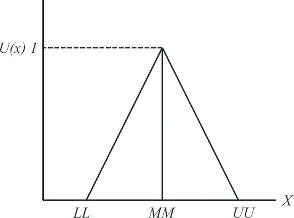
In this study, TFNs are used to present the preferences of one criterion over another. The structure of TFNs is shown in Figure 4 and the membership function is show in Table 1. This study employs FAHP to conduct fuzzy hierarchical analysis by allowing TFNs for pair-wise comparisons and calculating the fuzzy preference weights. The evaluation processes of FAHP are, as follows.
Triangular fuzzy numbers.
| Fuzzy Number | Linguistic Scale | Scale of Triangular Fuzzy Conversation | Scale of Triangular Fuzzy Reciprocal |
|---|---|---|---|
| 9 | Perfect | (8, 9, 9) | (1/9, 1/9, 1/8) |
| 8 | Absolute | (7, 8, 9) | (1/9, 1/8, 1/7) |
| 7 | Very good | (6, 7, 8) | (1/8, 1/7, 1/6) |
| 6 | Fairly good | (5, 6, 7) | (1/7, 1/6, 1/5) |
| 5 | Good | (4, 5, 6) | (1/6, 1/5, 1/4) |
| 4 | Preferable | (3, 4, 5) | (1/5, 1/4, 1/3) |
| 3 | Not bad | (2, 3, 4) | (1/4, 1/3, 1/2) |
| 2 | Weak advantage | (1, 2, 3) | (1/3, 1/2, 1) |
| 1 | Equal | (1, 1, 2) | (1, 1, 1) |
Process 1: Construct the Problem and Model
The problem should be clearly declared and decomposed into a rational system such as a network. The structure can be obtained according to the opinion of decision makers through the modified Delphi method, brainstorming, or other appropriate methods.
This study collected the sub-criteria, as based on literature review and expert interviews, and used a Likert 7-point scale for scoring, which ranges from very important (7) to very unimportant (1). After obtaining the scores, consistency testing was conducted using quartile deviation (QD) to sort the criteria. The criteria with a score of 4.00 or below and a QD below 1.00 were deleted; while the others were retained. As there is a large amount of data, debt-paying ability (DA) is used as an example to describe the details.
Process 2: Construct the TFNs
As each number in the pair-wise comparison matrix represents the subjective opinion of decision makers and is an ambiguous concept, fuzzy numbers work best to consolidate fragmented expert opinions through TFNs and the membership function of the linguistic scale (see Table 1). The TFNs
Process 3: Construct the Fuzzy Pair-wise Comparison Matrix
Saaty [42] argued that the geometric mean accurately represents the consensus of experts, and thus, it is most widely used in practical applications. In this study, the geometric mean method is used as the model for TFNs.
According to expert opinion and linguistic scale transformation, construct the TFNs of
Establish fuzzy pair-wise comparison matrix
Process 4: Computation of the Fuzzy Weights
In order to calculate the local weights of each element in
Process 5: Defuzzification
While various Defuzzification methods are available, the method adopted herein is derived from Yager [64], meaning a centroid defuzzification method called the center of gravity. In the case of TFNs, the translating formulae is [65]:
Process 6: Normalization
As the summation of the defuzzification weights of each criterion is not equal to 1, it must normalize the defuzzification weights to a new weight (NW). The equation of the NW is:
3. EMPIRICAL STUDY
This study developed a methodology to evaluate the optimal CO in the supply chain of the smartphone industry according to the opinions of experts employed in the financial field. The framework is shown in Figure 5. This evaluation model is constructed based on the FAHP algorithm to assess the optimal CO in the supply chain of the smartphone industry, which comprises the following processes:
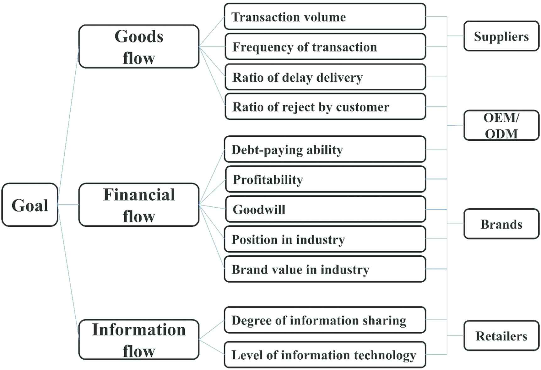
Hierarchical structure to evaluate the optimal CO in smartphone supply chain for financer.
Process 1: Construct the Problem and Model
According to Ali-Yrkko et al. [18] and Linden et al. [19], a general consensus among experts must be reached in order to construct a framework. The final goal of evaluating the ideal CO in the smartphone supply chain industry for the financial sector can thus be achieved, followed by three-evaluation criteria, eleven sub-criteria, and finally, the alternatives (Figure 5).
The evaluation criteria and sub-criteria used to determine the CO are defined, as follows:
Goods flow (GF) includes four sub-criteria, for example, transaction volume, frequency of transactions, ratio of delayed delivery, and ratio of being rejected by customers.
Transaction volume (TV): The total amount of transactions completed and logged in a specific time period.
Frequency of transactions (FT): The number of transaction occurrences in a given time period.
Ratio of delayed delivery (RDD): The number of transactions where delivery was delayed due to problems unrelated to logistics, as compared to the number of transactions where delivery was completed within the agreed upon time frame.
Ratio of being rejected by customers (RRC): The number of transactions where delivery was accepted by the customer, as compared to the number of transactions where the delivery was rejected by the customer.
FF includes five sub-criteria: DA, profitability, goodwill, position in the industry, and brand value in the industry.
Debt-paying ability (DA): The ability of the company to repay its debt obligations.
Profitability Analysis (PA): The company's income after input costs, expenses, and other obligations are paid.
Goodwill (GW): The value of the company beyond its assets and liabilities.
Position in industry (PII): A qualitative assessment of where a company stands in the specific industry relative to other operations in the supply chain.
Brand value in industry (BVI): A qualitative assessment of a company's brand when compared to others in the industry.
Information flow (IF) includes three sub-criteria: degree of information sharing, level of information technology, and degree of integrating all enterprise information systems (EIS).
Degree of information sharing (DIS): The level of sharing transaction records between all members of the supply chain.
Level of information technology (LIT): The degree to which a company integrates efficiency by increasing its computerized systems.
Process 2: Construct the TFNs
This study developed the TFNs (see Figure 4) of each pair-wise comparison through the fuzzy linguistic scale, and then, established the TFNs using Equations (7–10). Each expert made a pair-wise comparison of the decision criteria and gave them relative scores; Tables 2 and 3 show a sample of the first expert's pair-wise comparison scores and fuzzy linguistic pair-wise matrix, which is in line with the goal of the criteria (1 tier). Tables 4 and 5 show a sample of the first expert's pair-wise comparison scores and fuzzy linguistic pair-wise matrix criterion of the GF, which is in line with the goal of the sub-criteria (2 tier). Tables 6 and 7 show a sample of the first expert's pair-wise comparison scores and fuzzy linguistic pair-wise matrix in the sub-criterion of TV, which is in line with the goal of the alternatives (3 tier).
| GF | FF | IF | |
|---|---|---|---|
| GF | 1.000 | 0.200 | 4.000 |
| FF | 5.000 | 1.000 | 8.000 |
| IF | 0.250 | 0.125 | 1.000 |
The pair-wise comparison matrix of goal with criteria.
| Goal | GF | FF | IF |
|---|---|---|---|
| GF | (1.000 1.000 1.000) | (0.167 0.200 0.250) | (3.000 4.000 5.000) |
| FF | (4.000 5.000 6.000) | (1.000 1.000 1.000) | (7.000 8.000 9.000) |
| IF | (0.200 0.250 0.333) | (0.111 0.125 0.143) | (1.000 1.000 1.000) |
The fuzzy linguistic scale of goal with criteria.
| GF | TV | FT | RDD | RRC |
|---|---|---|---|---|
| TV | 1.000 | 2.000 | 2.000 | 0.333 |
| FT | 0.500 | 1.000 | 3.000 | 0.200 |
| RDD | 0.500 | 0.333 | 1.000 | 0.167 |
| RRC | 3.000 | 5.000 | 6.000 | 1.000 |
The pair-wise comparison matrix of GF criterion with sub-criteria.
| GF | TV | FT | RDD | RRC |
|---|---|---|---|---|
| TV | (1.000 1.000 1.000) | (1.000 2.000 3.000) | (1.000 2.000 3.000) | (0.250 0.333 0.500) |
| FT | (0.333 0.500 1.000) | (1.000 1.000 1.000) | (2.000 3.000 4.000) | (0.167 0.200 0.250) |
| RDD | (0.333 0.500 1.000) | (0.250 0.333 0.500) | (1.000 1.000 1.000) | (0.143 0.167 0.200) |
| RRC | (2.000 3.000 4.000) | (4.000 5.000 6.000) | (5.000 6.000 7.000) | (1.000 1.000 1.000) |
The fuzzy linguistic scale of GF criterion with sub-criteria.
| TV | Supplier | OEM/ODM | Brands | Retailer |
|---|---|---|---|---|
| Supplier | 1.000 | 0.200 | 0.167 | 1.000 |
| OEM/ODM | 5.000 | 1.000 | 0.200 | 2.000 |
| Brands | 6.000 | 5.000 | 1.000 | 6.000 |
| Retailer | 1.000 | 0.500 | 0.167 | 1.000 |
The pair-wise comparison matrix of sub-criterion of TV with alternatives.
| TV | Supplier | OEM/ODM | Brands | Retailer |
|---|---|---|---|---|
| Supplier | (1.000 1.000 1.000) | (0.167 0.200 0.250) | (0.143 0.167 0.200) | (1.000 1.000 1.000) |
| OEM/ODM | (4.000 5.000 6.000) | (1.000 1.000 1.000) | (0.167 0.200 0.250) | (1.000 2.000 3.000) |
| Brands | (5.000 6.000 7.000) | (4.000 5.000 6.000) | (1.000 1.000 1.000) | (5.000 6.000 7.000) |
| Retailer | (1.000 1.000 1.000) | (0.333 0.500 1.000) | (0.143 0.167 0.200) | (1.000 1.000 1.000) |
The fuzzy linguistic scale of sub-criterion of TV with alternatives.
Process 3: Construct the Fuzzy Pair-wise Comparison Matrix
Equations (11–15) are used to build the fuzzy pair-wise comparison matrix according to the results of TFNs from experts. All fuzzy pair-wise comparison matrixes of the criteria, sub-criteria, and alternatives are shown in Tables 8–11, respectively.
| Goal | GF | FF | IF | ||||||||||||
|---|---|---|---|---|---|---|---|---|---|---|---|---|---|---|---|
| GF | 1.000 | 1.000 | 1.000 | 0.687 | 0.841 | 1.107 | 1.225 | 1.807 | 2.475 | ||||||
| FF | 0.904 | 1.189 | 1.456 | 1.000 | 1.000 | 1.000 | 1.861 | 2.272 | 2.711 | ||||||
| IF | 0.404 | 0.553 | 0.816 | 0.369 | 0.440 | 0.537 | 1.000 | 1.000 | 1.000 | ||||||
| Note: R.I. = 0.580, Lambda max = 3.002, C.I. = 0.001, C.R. = 0.002 | |||||||||||||||
| GF | TV | FT | RDD | RRC | |||||||||||
| TV | 1.000 | 1.000 | 1.000 | 0.795 | 1.316 | 1.861 | 0.307 | 0.439 | 0.622 | 0.485 | 0.707 | 0.962 | |||
| FT | 0.537 | 0.760 | 1.257 | 1.000 | 1.000 | 1.000 | 0.420 | 0.577 | 0.841 | 0.537 | 0.752 | 0.984 | |||
| RDD | 1.607 | 2.280 | 3.254 | 1.190 | 1.732 | 2.379 | 1.000 | 1.000 | 1.000 | 0.765 | 0.955 | 1.189 | |||
| RRC | 1.039 | 1.414 | 2.060 | 1.016 | 1.330 | 1.861 | 0.841 | 1.047 | 1.307 | 1.000 | 1.000 | 1.000 | |||
| Note: R.I. = 0.890, Lambda max = 4.049, C.I. = 0.016, C.R. = 0.018 | |||||||||||||||
| FF | DA | PA | GW | PII | BVI | ||||||||||
| DA | 1.000 | 1.000 | 1.000 | 0.343 | 0.455 | 0.639 | 1.107 | 1.506 | 1.911 | 0.639 | 0.874 | 1.144 | 0.577 | 0.740 | 0.919 |
| PA | 1.565 | 2.198 | 2.913 | 1.000 | 1.000 | 1.000 | 1.848 | 2.317 | 2.817 | 1.720 | 2.378 | 3.118 | 1.000 | 1.607 | 2.280 |
| GW | 0.523 | 0.664 | 0.904 | 0.355 | 0.432 | 0.541 | 1.000 | 1.000 | 1.000 | 0.841 | 1.414 | 2.060 | 0.522 | 0.783 | 1.144 |
| PII | 0.874 | 1.144 | 1.565 | 0.321 | 0.420 | 0.581 | 0.485 | 0.707 | 1.189 | 1.000 | 1.000 | 1.000 | 0.261 | 0.359 | 0.595 |
| BVI | 1.088 | 1.351 | 1.732 | 0.439 | 0.622 | 1.000 | 0.874 | 1.278 | 1.917 | 1.682 | 2.783 | 3.834 | 1.000 | 1.000 | 1.000 |
| Note: R.I. = 1.110, Lambda max = 5.106, C.I. = 0.026, C.R. = 0.024 | |||||||||||||||
| IF | DIS | LIT | |||||||||||||
| DIS | 1.000 | 1.000 | 1.000 | 1.000 | 1.210 | 1.414 | |||||||||
| LIT | 0.707 | 0.827 | 1.000 | 1.000 | 1.000 | 1.000 | |||||||||
| Note: R.I. = 0.000, Lambda max = 2.000, C.I. = 0.000, C.R. = 0.000 | |||||||||||||||
The fuzzy pair-wise comparison matrix of criteria and sub-criteria.
| TV | Supplier | OEM/ODM | Brands | Retailer | ||||||||
|---|---|---|---|---|---|---|---|---|---|---|---|---|
| Supplier | 1.000 | 1.000 | 1.000 | 0.904 | 1.414 | 1.917 | 0.467 | 0.669 | 0.880 | 2.632 | 3.201 | 3.722 |
| OEM/ODM | 0.522 | 0.707 | 1.107 | 1.000 | 1.000 | 1.000 | 0.439 | 0.523 | 0.615 | 1.316 | 2.000 | 2.590 |
| Brands | 1.136 | 1.495 | 2.141 | 1.627 | 1.911 | 2.280 | 1.000 | 1.000 | 1.000 | 2.432 | 3.130 | 3.708 |
| Retailer | 0.269 | 0.312 | 0.380 | 0.386 | 0.500 | 0.760 | 0.270 | 0.319 | 0.411 | 1.000 | 1.000 | 1.000 |
| Note: R.I. = 0.890, Lambda max = 4.015, C.I. = 0.005, C.R. = 0.006 | ||||||||||||
| FT | Supplier | OEM/ODM | Brands | Retailer | ||||||||
| Supplier | 1.000 | 1.000 | 1.000 | 1.861 | 2.913 | 3.936 | 0.620 | 0.726 | 0.856 | 1.189 | 1.682 | 2.178 |
| OEM/ODM | 0.254 | 0.343 | 0.537 | 1.000 | 1.000 | 1.000 | 0.333 | 0.485 | 0.633 | 0.962 | 1.189 | 1.414 |
| Brands | 1.169 | 1.377 | 1.613 | 1.579 | 2.060 | 3.002 | 1.000 | 1.000 | 1.000 | 2.632 | 3.834 | 4.821 |
| Retailer | 0.459 | 0.595 | 0.841 | 0.707 | 0.841 | 1.039 | 0.207 | 0.261 | 0.380 | 1.000 | 1.000 | 1.000 |
| Note: R.I. = 0.890, Lambda max = 4.090, C.I. = 0.030, C.R. = 0.034 | ||||||||||||
| RDD | Supplier | OEM/ODM | Brands | Retailer | ||||||||
| Supplier | 1.000 | 1.000 | 1.000 | 0.572 | 0.816 | 1.107 | 0.841 | 1.414 | 2.060 | 1.000 | 1.480 | 1.968 |
| OEM/ODM | 0.904 | 1.225 | 1.748 | 1.000 | 1.000 | 1.000 | 1.136 | 1.565 | 1.968 | 0.946 | 1.456 | 2.000 |
| Brands | 0.485 | 0.707 | 1.189 | 0.508 | 0.639 | 0.880 | 1.000 | 1.000 | 1.000 | 0.408 | 0.639 | 0.895 |
| Retailer | 0.508 | 0.676 | 1.000 | 0.500 | 0.687 | 1.057 | 1.117 | 1.565 | 2.449 | 1.000 | 1.000 | 1.000 |
| Note: R.I. = 0.890, Lambda max = 4.028, C.I. = 0.009, C.R. = 0.010 | ||||||||||||
| RRC | Supplier | OEM/ODM | Brands | Retailer | ||||||||
| Supplier | 1.000 | 1.000 | 1.000 | 1.520 | 2.178 | 3.130 | 1.065 | 1.520 | 1.968 | 0.447 | 0.707 | 1.000 |
| OEM/ODM | 0.319 | 0.459 | 0.658 | 1.000 | 1.000 | 1.000 | 1.074 | 1.414 | 1.778 | 0.502 | 0.676 | 0.847 |
| Brands | 0.508 | 0.658 | 0.939 | 0.562 | 0.707 | 0.931 | 1.000 | 1.000 | 1.000 | 0.500 | 0.615 | 0.760 |
| Retailer | 1.000 | 1.414 | 2.236 | 1.181 | 1.480 | 1.992 | 1.317 | 1.627 | 2.000 | 1.000 | 1.000 | 1.000 |
| Note: R.I. = 0.890, Lambda max = 4.074, C.I. = 0.025, C.R. = 0.028 | ||||||||||||
The fuzzy pair-wise comparison matrix of each criterion in GF of alternatives.
| DA | Supplier | OEM/ODM | Brands | Retailer | ||||||||
|---|---|---|---|---|---|---|---|---|---|---|---|---|
| Supplier | 1.000 | 1.000 | 1.000 | 1.316 | 2.378 | 3.409 | 0.869 | 1.316 | 1.760 | 0.669 | 0.880 | 1.136 |
| OEM/ODM | 0.293 | 0.420 | 0.760 | 1.000 | 1.000 | 1.000 | 0.687 | 0.931 | 1.300 | 0.731 | 0.955 | 1.245 |
| Brands | 0.568 | 0.760 | 1.150 | 0.769 | 1.075 | 1.456 | 1.000 | 1.000 | 1.000 | 0.795 | 1.107 | 1.414 |
| Retailer | 0.880 | 1.136 | 1.495 | 0.803 | 1.047 | 1.368 | 0.707 | 0.904 | 1.257 | 1.000 | 1.000 | 1.000 |
| Note: R.I. = 0.890, Lambda max = 4.090, C.I. = 0.030, C.R. = 0.034 | ||||||||||||
| PA | Supplier | OEM/ODM | Brands | Retailer | ||||||||
| Supplier | 1.000 | 1.000 | 1.000 | 0.532 | 0.783 | 1.075 | 0.522 | 0.639 | 0.773 | 1.075 | 1.732 | 2.632 |
| OEM/ODM | 0.931 | 1.278 | 1.880 | 1.000 | 1.000 | 1.000 | 0.439 | 0.508 | 0.595 | 1.236 | 1.633 | 2.027 |
| Brands | 1.294 | 1.565 | 1.917 | 1.682 | 1.968 | 2.280 | 1.000 | 1.000 | 1.000 | 1.682 | 2.060 | 2.280 |
| Retailer | 0.380 | 0.577 | 0.931 | 0.493 | 0.612 | 0.809 | 0.439 | 0.485 | 0.595 | 1.000 | 1.000 | 1.000 |
| Note: R.I. = 0.890, Lambda max = 4.037, C.I. = 0.012, C.R. = 0.014 | ||||||||||||
| GW | Supplier | OEM/ODM | Brands | Retailer | ||||||||
| Supplier | 1.000 | 1.000 | 1.000 | 0.537 | 0.760 | 1.106 | 0.236 | 0.319 | 0.517 | 1.189 | 1.565 | 1.861 |
| OEM/ODM | 0.904 | 1.316 | 1.862 | 1.000 | 1.000 | 1.000 | 0.280 | 0.334 | 0.435 | 0.604 | 0.931 | 1.414 |
| Brands | 1.935 | 3.131 | 4.243 | 2.300 | 2.991 | 3.568 | 1.000 | 1.000 | 1.000 | 2.141 | 2.828 | 3.409 |
| Retailer | 0.537 | 0.639 | 0.841 | 0.707 | 1.075 | 1.655 | 0.293 | 0.354 | 0.467 | 1.000 | 1.000 | 1.000 |
| Note: R.I. = 0.890, Lambda max = 4.062, C.I. = 0.021, C.R. = 0.023 | ||||||||||||
| PII | Supplier | OEM/ODM | Brands | Retailer | ||||||||
| Supplier | 1.000 | 1.000 | 1.000 | 0.343 | 0.455 | 0.639 | 1.075 | 1.495 | 1.894 | 2.213 | 3.224 | 4.229 |
| OEM/ODM | 1.565 | 2.198 | 2.913 | 1.000 | 1.000 | 1.000 | 1.047 | 1.627 | 2.213 | 4.281 | 5.384 | 6.447 |
| Brands | 0.528 | 0.669 | 0.931 | 0.452 | 0.615 | 0.955 | 1.000 | 1.000 | 1.000 | 1.278 | 1.732 | 2.280 |
| Retailer | 0.236 | 0.310 | 0.452 | 0.155 | 0.186 | 0.234 | 0.439 | 0.577 | 0.783 | 1.000 | 1.000 | 1.000 |
| Note: R.I. = 0.890, Lambda max = 4.065, C.I. = 0.022, C.R. = 0.024 | ||||||||||||
| BVI | Supplier | OEM/ODM | Brands | Retailer | ||||||||
| Supplier | 1.000 | 1.000 | 1.000 | 0.880 | 1.414 | 1.968 | 0.390 | 0.481 | 0.639 | 1.732 | 2.378 | 2.943 |
| OEM/ODM | 0.508 | 0.707 | 1.136 | 1.000 | 1.000 | 1.000 | 0.355 | 0.439 | 0.595 | 1.682 | 2.783 | 3.834 |
| Brands | 1.565 | 2.079 | 2.564 | 1.682 | 2.280 | 2.818 | 1.000 | 1.000 | 1.000 | 1.934 | 2.631 | 3.319 |
| Retailer | 0.340 | 0.420 | 0.577 | 0.261 | 0.359 | 0.595 | 0.301 | 0.380 | 0.517 | 1.000 | 1.000 | 1.000 |
| Note: R.I. = 0.890, Lambda max = 4.094, C.I. = 0.031, C.R. = 0.035 | ||||||||||||
The fuzzy pair-wise comparison matrix of each criterion in FF of alternatives.
| DIS | Supplier | OEM/ODM | Brands | Retailer | ||||||||
|---|---|---|---|---|---|---|---|---|---|---|---|---|
| Supplier | 1.000 | 1.000 | 1.000 | 0.707 | 0.760 | 0.841 | 1.000 | 1.316 | 1.627 | 3.027 | 4.120 | 5.180 |
| OEM/ODM | 1.190 | 1.316 | 1.414 | 1.000 | 1.000 | 1.000 | 0.955 | 1.245 | 1.514 | 3.464 | 4.527 | 5.566 |
| Brands | 0.615 | 0.760 | 1.000 | 0.661 | 0.803 | 1.047 | 1.000 | 1.000 | 1.000 | 1.778 | 2.449 | 3.027 |
| Retailer | 0.193 | 0.243 | 0.330 | 0.180 | 0.221 | 0.289 | 0.330 | 0.408 | 0.562 | 1.000 | 1.000 | 1.000 |
| Note: R.I. = 0.890, Lambda max = 4.022, C.I. = 0.007, C.R. = 0.008 | ||||||||||||
| LIT | Supplier | OEM/ODM | Brands | Retailer | ||||||||
| Supplier | 1.000 | 1.000 | 1.000 | 0.355 | 0.452 | 0.615 | 1.026 | 1.414 | 1.800 | 1.414 | 1.968 | 2.632 |
| OEM/ODM | 1.627 | 2.213 | 2.817 | 1.000 | 1.000 | 1.000 | 1.189 | 1.565 | 1.917 | 3.201 | 4.427 | 5.544 |
| Brands | 0.556 | 0.707 | 0.974 | 0.522 | 0.639 | 0.841 | 1.000 | 1.000 | 1.000 | 1.934 | 2.632 | 3.224 |
| Retailer | 0.380 | 0.508 | 0.707 | 0.180 | 0.226 | 0.312 | 0.310 | 0.380 | 0.517 | 1.000 | 1.000 | 1.000 |
| Note: R.I. = 0.890, Lambda max = 4.056, C.I. = 0.019, C.R. = 0.021 | ||||||||||||
The fuzzy pair-wise comparison matrix of each criterion in IF of alternatives.
Process 4: Computation of the Fuzzy Weights
The results are calculated from the fuzzy pair-wise comparison matrix into fuzzy weights
The fuzzy weights of the criteria, sub-criteria, and alternatives are shown in Table 12.
| Goal |
GF |
FF |
IF |
||||||||||||
|---|---|---|---|---|---|---|---|---|---|---|---|---|---|---|---|
| Goal | LL | MM | UU | TV | LL | MM | UU | DA | LL | MM | UU | DIS | LL | MM | UU |
| GF | 0.252 | 0.363 | 0.525 | Supplier | 0.191 | 0.297 | 0.436 | Supplier | 0.181 | 0.317 | 0.511 | Supplier | 0.228 | 0.312 | 0.422 |
| FF | 0.318 | 0.440 | 0.593 | OEM/ODM | 0.138 | 0.208 | 0.317 | OEM/ODM | 0.120 | 0.192 | 0.333 | OEM/ODM | 0.266 | 0.361 | 0.480 |
| IF | 0.142 | 0.197 | 0.285 | Brands | 0.270 | 0.389 | 0.568 | Brands | 0.148 | 0.240 | 0.392 | Brands | 0.174 | 0.242 | 0.345 |
| Retailer | 0.076 | 0.106 | 0.162 | Retailer | 0.162 | 0.251 | 0.400 | Retailer | 0.062 | 0.084 | 0.124 | ||||
| GF | LL | MM | UU | FT | LL | MM | UU | PA | LL | MM | UU | LIT | LL | MM | UU |
| TV | 0.111 | 0.193 | 0.316 | Supplier | 0.199 | 0.308 | 0.456 | Supplier | 0.147 | 0.229 | 0.347 | Supplier | 0.154 | 0.233 | 0.356 |
| FT | 0.112 | 0.183 | 0.311 | OEM/ODM | 0.098 | 0.150 | 0.231 | OEM/ODM | 0.167 | 0.241 | 0.351 | OEM/ODM | 0.287 | 0.436 | 0.637 |
| RDD | 0.208 | 0.337 | 0.536 | Brands | 0.273 | 0.407 | 0.609 | Brands | 0.275 | 0.377 | 0.508 | Brands | 0.157 | 0.230 | 0.347 |
| RRC | 0.184 | 0.286 | 0.461 | Retailer | 0.094 | 0.135 | 0.210 | Retailer | 0.106 | 0.153 | 0.234 | Retailer | 0.069 | 0.101 | 0.158 |
| FF | LL | MM | UU | RDD | LL | MM | UU | GW | LL | MM | UU | ||||
| DA | 0.098 | 0.159 | 0.256 | Supplier | 0.156 | 0.279 | 0.467 | Supplier | 0.111 | 0.172 | 0.283 | ||||
| PA | 0.199 | 0.338 | 0.550 | OEM/ODM | 0.186 | 0.316 | 0.519 | OEM/ODM | 0.111 | 0.176 | 0.289 | ||||
| GW | 0.088 | 0.148 | 0.251 | Brands | 0.106 | 0.179 | 0.315 | Brands | 0.312 | 0.498 | 0.748 | ||||
| PII | 0.074 | 0.123 | 0.223 | Retailer | 0.137 | 0.226 | 0.407 | Retailer | 0.103 | 0.154 | 0.251 | ||||
| BVI | 0.135 | 0.232 | 0.405 | ||||||||||||
| IF | LL | MM | UU | RRC | LL | MM | UU | PII | LL | MM | UU | ||||
| TV | 0.457 | 0.547 | 0.646 | Supplier | 0.177 | 0.299 | 0.478 | Supplier | 0.165 | 0.261 | 0.409 | ||||
| FT | 0.384 | 0.453 | 0.543 | OEM/ODM | 0.124 | 0.197 | 0.303 | OEM/ODM | 0.282 | 0.450 | 0.691 | ||||
| Brands | 0.118 | 0.177 | 0.274 | Brands | 0.129 | 0.197 | 0.324 | ||||||||
| Retailer | 0.215 | 0.328 | 0.524 | Retailer | 0.062 | 0.092 | 0.146 | ||||||||
| BVI | LL | MM | UU | ||||||||||||
| Supplier | 0.159 | 0.253 | 0.393 | ||||||||||||
| OEM/ODM | 0.134 | 0.216 | 0.360 | ||||||||||||
| Brands | 0.272 | 0.421 | 0.627 | ||||||||||||
| Retailer | 0.073 | 0.110 | 0.184 | ||||||||||||
The fuzzy weights of all elements.
Process 5: Defuzzification
After computation of the fuzzy weights, defuzzification is required to estimate the real weights of Eq. (17). Defuzzification is performed on the samples of criteria GF, FF, and IF to calculate the real weights, as follows.
The real weights of all elements are show in Table 13.
| Goal (Level 2) |
Criteria (Level 3) |
GF (Alternatives) |
FF (Alternatives) |
IF (Alternatives) |
|||||
|---|---|---|---|---|---|---|---|---|---|
| Weights | GF | Weights | TV | Weights | DA | Weights | DIS | Weights | |
| GF | 0.380 | TV | 0.207 | Supplier | 0.308 | Supplier | 0.336 | Supplier | 0.321 |
| FF | 0.450 | FT | 0.202 | OEM/ODM | 0.221 | OEM/ODM | 0.215 | OEM/ODM | 0.369 |
| IF | 0.208 | RDD | 0.361 | Brands | 0.409 | Brands | 0.260 | Brands | 0.254 |
| RRC | 0.310 | Retailer | 0.115 | Retailer | 0.271 | Retailer | 0.090 | ||
| FF | Weights | FT | Weights | PA | Weights | LIT | Weights | ||
| DA | 0.171 | Supplier | 0.321 | Supplier | 0.241 | Supplier | 0.248 | ||
| PA | 0.362 | OEM/ODM | 0.160 | OEM/ODM | 0.253 | OEM/ODM | 0.453 | ||
| GW | 0.162 | Brands | 0.430 | Brands | 0.386 | Brands | 0.245 | ||
| PII | 0.140 | Retailer | 0.146 | Retailer | 0.164 | Retailer | 0.109 | ||
| BVI | 0.257 | ||||||||
| IF | Weights | RDD | Weights | GW | Weights | ||||
| TV | 0.550 | Supplier | 0.301 | Supplier | 0.189 | ||||
| FT | 0.460 | OEM/ODM | 0.341 | OEM/ODM | 0.192 | ||||
| Brands | 0.200 | Brands | 0.519 | ||||||
| Retailer | 0.256 | Retailer | 0.169 | ||||||
| RRC | Weights | PII | Weights | ||||||
| Supplier | 0.318 | Supplier | 0.278 | ||||||
| OEM/ODM | 0.208 | OEM/ODM | 0.474 | ||||||
| Brands | 0.189 | Brands | 0.217 | ||||||
| Retailer | 0.356 | Retailer | 0.100 | ||||||
| BVI | Weights | ||||||||
| Supplier | 0.268 | ||||||||
| OEM/ODM | 0.237 | ||||||||
| Brands | 0.440 | ||||||||
| Retailer | 0.122 | ||||||||
The real weights of all elements.
Process 6: Normalization
Finally, the summation of defuzzification weights is not equal to one in the same hierarchy; therefore, the defuzzification weights must be normalized by Eq. (18) to obtain the NWs, as follows:
The
| Criteria | Normalized | Sub-criteria | Normalized |
|---|---|---|---|
| GF | 0.366 | TV | 0.192 |
| FT | 0.187 | ||
| RDD | 0.334 | ||
| RRC | 0.287 | ||
| FF | 0.434 | DA | 0.156 |
| PA | 0.332 | ||
| GW | 0.148 | ||
| PII | 0.128 | ||
| BVI | 0.236 | ||
| IF | 0.200 | TV | 0.545 |
| FT | 0.455 |
The
| TV | Normalized | DA | Normalized | DIS | Normalized |
|---|---|---|---|---|---|
| Supplier | 0.292 | Supplier | 0.311 | Supplier | 0.310 |
| OEM/ODM | 0.210 | OEM/ODM | 0.199 | OEM/ODM | 0.357 |
| Brands | 0.389 | Brands | 0.240 | Brands | 0.245 |
| Retailer | 0.109 | Retailer | 0.250 | Retailer | 0.087 |
| FT | PA | LIT | |||
| Supplier | 0.304 | Supplier | 0.231 | Supplier | 0.235 |
| OEM/ODM | 0.151 | OEM/ODM | 0.242 | OEM/ODM | 0.430 |
| Brands | 0.407 | Brands | 0.370 | Brands | 0.232 |
| Retailer | 0.138 | Retailer | 0.157 | Retailer | 0.104 |
| RDD | GW | ||||
| Supplier | 0.274 | Supplier | 0.177 | ||
| OEM/ODM | 0.310 | OEM/ODM | 0.179 | ||
| Brands | 0.182 | Brands | 0.486 | ||
| Retailer | 0.234 | Retailer | 0.158 | ||
| RRC | PII | ||||
| Supplier | 0.297 | Supplier | 0.260 | ||
| OEM/ODM | 0.194 | OEM/ODM | 0.443 | ||
| Brands | 0.177 | Brands | 0.203 | ||
| Retailer | 0.332 | Retailer | 0.093 | ||
| BVI | |||||
| Supplier | 0.251 | ||||
| OEM/ODM | 0.222 | ||||
| Brands | 0.412 | ||||
| Retailer | 0.115 | ||||
The
Table 16 shows the FAHP synthesis results regarding the evaluation of the CO in the supply chain of the smartphone industry: Supplier (0.287), OEM/ODM (0.256), Brands (0.298), and Retailer (0.159). Thus, the sequential weights of the four operations of the smartphone supply chain are Brands > Supplier > OEM/ODM > Retailer. The sequential weights of the 11 criteria are PA > RDD > DIS > RRC > BVI, and so on.
| Fuzzy AHP Synthesis Value |
||||||||||||
|---|---|---|---|---|---|---|---|---|---|---|---|---|
| Goal | Criteria | Local Weights | Global Weights | Rank | Sub-Criteria | Local Weights | Global Weights | Rank | Alternatives | Local Weights | Global Weights | Rank |
| G | GF | 0.380 | 0.366 | 2 | TV | 0.192 | 0.070 | 7 | Supplier | 0.267 | 0.287 | 2 |
| FT | 0.187 | 0.068 | 8 | OEM/ODM | 0.239 | 0.256 | 3 | |||||
| RDD | 0.334 | 0.122 | 2 | Brands | 0.279 | 0.298 | 1 | |||||
| RRC | 0.287 | 0.105 | 4 | Retailer | 0.148 | 0.159 | 4 | |||||
| FF | 0.450 | 0.434 | 1 | DA | 0.156 | 0.068 | 9 | |||||
| PA | 0.332 | 0.144 | 1 | |||||||||
| GW | 0.148 | 0.064 | 10 | |||||||||
| PII | 0.128 | 0.056 | 11 | |||||||||
| BVI | 0.236 | 0.102 | 5 | |||||||||
| IF | 0.208 | 0.200 | 3 | DIS | 0.545 | 0.109 | 3 | |||||
| LIT | 0.455 | 0.091 | 6 | |||||||||
The fuzzy AHP synthesis value of criteria, sub-criteria, and alternatives.
Therefore, the CO is “brand,” meaning when a potential financer wants to provide SCF services to the supply chain of the smartphone industry, it should focus on the “brand” of the company. The company can provide the financer with the purchase records, which will result in the delivery of credit, transaction records, invoices, and so on, to their upstream (OEM/ODM and supplier) companies.
In addition, the “Brand” company can provide shipment records to the financer, which would result in the delivery of credit, transaction records, invoices, and so on, to their downstream (Retailer). These activities can improve the efficiency of accounts receivable financing for firms upstream of the Brand company, and enhance the accounts payable financing efficiency for firms downstream of the Brand company in the smartphone industry supply chain ecosystem. Moreover, it can elevate the operating income, operating scale, market share, services, innovation commodities, and so on, for the financer.
While the implementation of the SCF concept can upgrade the FF for the supply chain of the smartphone industry and improve the operations of the financer, the financer must consider many risks during implementation. From the three flows of smartphone SCM, the critical criterion of evaluating CO in SCF is “FF,” and some key sub-criteria are “PA,” “RDD,” “DIS,” “RRC,” and “BVI,” meaning when a financer provides SCF to smartphone industry supply chain, the FF, PA, RDD, DIS, RRC, and BVI are the most important, and smartphone industry supply chain members should focus on the performance of these indicators.
Therefore, the results of the application of the FAHP model demonstrate that the financer must evaluate the CO according to the SCF services for the smartphone industry, meaning “Brand,” when it plans to provide SCF to the supply chain of the smartphone industry.
4. CONCLUSION
The development of a globalized economy has led to intense market competition, which has led to many industries implementing SCM as well as manufacturing, logistics, and marketing activities to coordinate the flow of goods, services, and money between the separate stages of an industry's supply chain, thus, FFs are important to all industries when implementing supply chain activities. SCF is new type of financial service that can enhance the financial efficiency of a supply chain, as the key concept of SCF is the delivery of credit. Using the transaction records of the CO, the financer will be able to provide a higher level of cash flow to the SMEs of supply chain. Moreover, SCF inherits numerous risks through the CO to upstream and downstream members in a supply chain ecosystem. These risks include supply chain systematic risk, transaction risk, bankruptcy risk, and so on. Nevertheless, applying with implementing the optimal CO in smartphone industry supply chain is a highly intricate topic for financial institution managers, administrators as well as decision makers.
As such, this study presents an evaluation framework that applies a combination of fuzzy analysis and AHP in the decision-making process to assess CO for acquiring the optimal operation in the smartphone industry supply chain for financial sectors. This framework comprises the fuzzy theory and AHP, which can solve the inherent uncertainties and imprecisions associated within the research model and obtain the relative weights in the fuzzy concept. The decision maker of financiers usually lack of the procedures of fuzzy objective decision-making to acquire the optimal CO in a supply chain and there are highly risks for providing the SCF into the supply chain process. FAHP is able to resolve the inherent uncertainties and imprecisions in all factors, thus making it a valid instrument for the decision maker to obtain an accurate alternative.
The results of this study show that the critical factors are “PA,” “RDD,” and “DIS” and the optimal CO is “Brand,” which means that when a financial sector provides SCF services to the supply chain of the smartphone industry ecosystem, “PA” is the one of important indicators, as it represents a company's revenue after operation costs, expenses, and other obligations have been met. PA points out the importance of profitability for the company. When the PA of the CO in the supply chain is low, it is unable to enhance the financial efficiency of other supply chain members. The lower the PA, the lower the level of lending by a financial institution; thus, PA is an important index of the financial constitution of a CO. The RDD means the efficiency of the ratio of delay delivery on brand operation is lower than others and the DIS on brand operation is higher than other members. The DIS includes information such as customers’ demand data, ordering data, and transaction data, and so on. Accordingly, the sharing on brand is more transparent than that for the supplier, manufacturer, and retailer in the supply chain. In the smartphone industry, the architecture of the smartphone industry supply chain is a highly complex environment. All of the products in the upstream to midstream must be processed via the brand. In other words, the different brands include different values in customer perception that will affect the sales volume and influence the profitability. Hence, financiers would providing SCF services to the smartphone industry should focus on the CO of “Brand,” and then, extend the loan level and improve the financial efficiency of the relative members in their supply chain.
Therefore, the proposed FAHP-based framework on decision-making is able to help by prioritizing and weighing the complex scenarios that assist the financial sectors in providing the SCF service involved in assessing the CO. This framework can provide academic support to administrators for financial institutions with a valuable guide for measuring the CO of the smartphone industry supply chain and acquiring the optimal solution in SCF service.
CONFLICT OF INTEREST
The authors declare they have no conflicts of interest.
AUTHORS' CONTRIBUTIONS
Research design, literature review, data collection, data analysis and manuscript writing are all conducted by Chun Yueh Lin.
ACKNOWLEDGEMENTS
This research was supported by Taiwan's Ministry of Science and Technology under grant 107-2410-H-034-006.
REFERENCES
Cite this article
TY  - JOUR
AU  - Chun-Yueh Lin
PY  - 2020
DA  - 2020/03/04
TI  - Optimal Core Operation in Supply Chain Finance Ecosystem by Integrating the Fuzzy Algorithm and Hierarchical Framework
JO  - International Journal of Computational Intelligence Systems
SP  - 259
EP  - 274
VL  - 13
IS  - 1
SN  - 1875-6883
UR  - https://doi.org/10.2991/ijcis.d.200226.001
DO  - 10.2991/ijcis.d.200226.001
ID  - Lin2020
ER  -