
Feature Selection Based on a Novel Improved Tree Growth Algorithm
- DOI
- 10.2991/ijcis.d.200219.001How to use a DOI?
- Keywords
- Feature selection; Tree growth algorithm; Evolutionary population dynamics; Metaheuristic
- Abstract
Feature selection plays a significant role in the field of data mining and machine learning to reduce the data dimension, speed up the model building process and improve algorithm performance. Tree growth algorithm (TGA) is a recent proposed population-based metaheuristic, which shows great power of search ability in solving optimization of continuous problems. However, TGA cannot be directly applied to feature selection problems. Also, we find that its efficiency still leave room for improvement. To tackle this problem, in this study, a novel improved TGA (iTGA) is proposed, which can resolve the feature selection problem efficiently. The main contribution includes, (1) a binary TGA is proposed to tackle the feature selection problems, (2) a linearly increasing parameter tuning mechanism is proposed to tune the parameter in TGA, (3) the evolutionary population dynamics (EPD) strategy is applied to improve the exploration and exploitation capabilities of TGA, (4) the efficiency of iTGA is evaluated on fifteen UCI benchmark datasets, the comprehensive results indicate that iTGA can resolve feature selection problems efficiently. Furthermore, the results of comparative experiments also verify the superiority of iTGA compared with other state-of-the-art methods.
- Copyright
- © 2020 The Authors. Published by Atlantis Press SARL.
- Open Access
- This is an open access article distributed under the CC BY-NC 4.0 license (http://creativecommons.org/licenses/by-nc/4.0/).
1. INTRODUCTION
In the last few decades, the amount of data generated from various industries have had a dramatic increase. Efficient and practical technology is extremely needed to find useful information from massive data and to turn such data into valuable knowledge, which leads to the rise of machine learning and data mining. The goal of data mining is to extract or generate well-organized knowledge from huge amounts of data through a series of processes including data cleaning, data integration, data reduction, data transformation [1]. In data mining, real-world applications usually contain a great number of features, and not all features are useful since some of them are redundant or irrelevant which will bring in poor performance of an algorithm [2]. Feature Selection plays a substantial role in data preprocessing that tries to select the most appropriate feature subset from the feature space by excluding the redundant and irrelevant features [3]. Feature selection can decrease the data dimension by removing irrelevant features, thereby speeding up the model building process and improving algorithm performance.
A few literature have discussed the topic of feature selection, and many methods have been proposed. These methods can be roughly divided into two main categories from the aspect of evaluation: the filter methods and the wrapper methods [4,5]. In filter-based approach, some data-reliant criteria are used for estimating a feature or a feature subset, and the learning algorithm is not involved in the process of feature selection [2]. The classical filter-based method includes correlation coefficient [6], information gain (IG) [7], Fisher score (F-score) criterion [8], ReliefF [9], correlation-based feature selection [10] and so on. In wrapper-based approach, a specific learning algorithm is utilized to assess the merit of a feature subset. Examples of common wrapper-based methods include sequential forward selection (SFS) [11], sequential backward selection (SBS) [12], sequential forward floating selection (SFFS) and sequential backward floating selection (SBFS) [13]. In general, the filter method usually requires less computational resources than the wrapper method since it does not involve any learning algorithms. However, it does not take into account the impact of each feature on the performance of the final classifier. The wrapper method fully investigated the classification performance to generate the best feature subset that represents the original features.
Selecting the appropriate feature subset from a high-dimensional feature space is a critical problem and it is very challenging. A few methods have been applied to solve this problem. Complete search method produces all feature subsets to choose the best one, which is impracticable for the high-dimensional feature space since a
Under this circumstances, the metaheuristics, which are well-regarded for their powerful global search ability, provide a new way to solve feature selection problems. In recent years, several nature-inspired metaheuristic methods have been utilized to figure out feature selection problems. Whale optimization algorithm (WOA) [14] is a recent nature-inspired metaheuristic, which has been successfully applied for tackling feature selection problems [15]. In addition, a new wrapper feature selection method based on the hybrid WOA embedded with simulation method was proposed [16]. Crow search algorithm (CSA) [17], a recently proposed metaheuristic that has been utilized to tackle feature selection problems as a wrapper-based approach [18]. Furthermore, A new fusion of grey wolf optimizer (GWO) [19] algorithm with a two-phase mutation was proposed [20] and successfully utilized to solve feature selection problems. Ant lion optimizer (ALO) [21], a recent population-based optimizer was applied as a searching approach in a wrapper feature selection method [22]. Besides, grasshopper optimization approach (GOA) [23] was utilized to handle feature selection problems [24] as a wrapper-based method. Moreover, a variant of the GOA was proposed [25] to solve feature selection problems. This approach has been enhanced by using evolutionary population dynamics (EPD) and selection operators in manipulating the whole population that eliminates and reposition poor individuals in the population to improve the whole population.
The majority of existing metaheuristics are modeled on direct observation of the special behavior of species. For example, The GOA inspired by the intelligent behaviors of grasshopper insects in nature. The ant colony optimization (ACO) [26] mimics the behavior of ants finding the shortest path between their colony and a source of food. These algorithms employ some evolutionary operators (pheromone accumulation mechanism in ACO) to each individual of a population to generate the next generation. However, such operators only consider the evolution of good individuals rather than the entire population [25]. On the contrary, EPD is another well-known evolutionary strategy, which aims to improve the population by eliminating poor solutions rather than directly improve good solutions [27]. Extremal optimization (EO) [28] is a metaheuristic based on EPD that has been successfully applied in many fields [29–31]. Furthermore, [25,27,32] show that EPD, as a controlling metaheuristic, is also useful to a variety of population-based algorithms to improve the algorithm performance.
Tree growth algorithm, TGA, is a recent nature-inspired population-based metaheuristic which mimics the growing behavior of tree in the jungle. The performance of TGA was evaluated on several well-known benchmarks and engineering problems [33]. The results in the author's reported show that the performance of TGA was very excellent and impressive. This motivated us to investigate the performance of TGA in the field of feature selection problems. Therefore, we presents a novel improved TGA (iTGA) for feature selection problem. In this work, we have made the following key contributions:
A binary TGA (BTGA) is proposed to tackle the feature selection problems.
A linearly increasing parameter tuning mechanism is proposed to tune the parameter to improve the local searchability of TGA.
The EPD strategy is applied to balance the exploration and exploitation capabilities of TGA.
The efficiency of iTGA has been evaluated and compared with serveal metaheuristics on 15 UCI benchmark datasets, the comprehensive results indicated that iTGA can resolve feature selection problems efficiently.
The rest of this paper is organized as follows: Section 2 gives a brief introduction of TGA. Section 3 presents the details of the proposed iTGA, and its application to feature selection problems. Section 4 describes and analyzes the performance of iTGA. Finally, in Section 5, conclusions and future works are given.
2. TREE GROWTH ALGORITHM
TGA is a recent nature-inspired population-based metaheuristic [33], which is inspired by the growing behavior of tree in the jungle. In TGA, a set of candidate solutions are randomly generated to construct the initial trees in the jungle. Next, the whole population of trees are divided into four groups according to their fitness value. Trees with better fitness will be assigned to the first group. In the first group, trees will grow further. The second group is called the competition for light group. In the second group, trees move to the position between the close best trees under different angles in order to reach the light. The third group is called the remove and replace group, which aims to replace the weak trees with new trees. The fourth group is the reproduction group, which are multiplied and created by the best trees. The detailed of TGA include four steps which is described below:
Step 1: the initial population of trees are randomly generated within a specified interval. Then, the population of trees are sorted based on their fitness value. The best
Step 2:
Step 3:
Step 4:
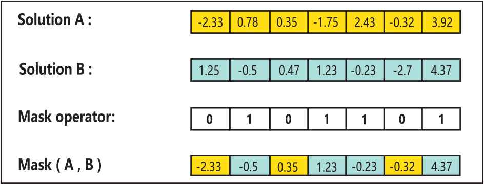
An example of mask operation.
In Figure 1, solution A is a new tree in
After that, the new trees in
3. THE IMPROVED TGA
As mentioned before, TGA has shown good performance in solving optimization of continuous problems. However, TGA cannot be directly applied to discrete optimization problems, such as, feature selection problem. In order to resolve feature selection problems with TGA, we proposed a novel iTGA algorithm. In iTGA, firstly, we proposed a BTGA to solve feature selection problems. Secondly, since TGA is sensitive to the parameter
3.1. BTGA for Feature Selection
As described earlier, feature selection is an NP-hard problem when
According to literature [34], one of the easiest ways to transform an algorithm from continues to the binary version without changing its basic structure is to utilize a transfer function. Therefore, we propose a new binarization method to transform the algorithm from continuous to discrete version. For every bit in the solution, we transform the continue value into discrete using Equation (7).
In feature selection, classification accuracy and number of selected features are two important evaluation criteria that should be taken into account in designing a fitness function. In this paper, the fitness function in Equation (9) is utilized to evaluate the selected subset which can well balance the classification accuracy and the number of selected features.
3.2. Linear Increasing Mechanism for Parameter Tuning
As discussed in Section 2, the parameter
Therefore, in this paper, we proposed a linearly increasing adaptive method to tune
3.3. Embedded TGA with EPD Strategy
EPD, also known as an evolution strategy, indicates that the population evolution can be achieved by eliminating the worst individuals and repositioning them around the best ones. The basis of EPD is established on the principle of self-organized criticality (SOC) [32], which points that a small change in individuals can influence the entire population and provide a delicate equilibrium without external forces [31]. It is observed that in the process of species evolution, evolution applies on the poor species as well [32]. In this case, the entire population quality is affected by eliminating the poor individuals. Several metaheuristics methods have successfully applied the strategy of EPD and SOC including EPD-based GOA algorithm [25], a self-organizing multi-objective evolutionary algorithm [35]. The EPD could be utilized as a controlling metaheuristic to improve the algorithm performance. The reason why EPD can improve the median of the entire population is that EPD strategy removes the worst individuals by repositioning them around the best ones.
As described earlier, the efficiency of TGA still leave room for improvement. Therefore, we introduce EPD into iTGA for improving the efficiency of TGA. In iTGA, the population was divided into two parts according to their fitness value. Half of the worst population is erased and repositioned around the best ones from the top half of the population.
According to the results of Talbi [36], however, “it means that using better solutions as initial solutions will not always lead to better local optima.” Because the best solutions may be biased during the search process, which leads to the imbalance statue of exploration and exploitation. For this reason, we cannot simply choose the best individual from the good half of the population, but apply a special selection mechanism to choose the individual from the top half of the population. For each individual in the poor half of the population, utilizing a selection operator to select an individual from the top half, and then do mask operation with the poor individual. Roulette wheel selection (RWS) [37] is a well-known selection technique that can be utilized in this work.
RWS, as well-known as fitness proportionate selection, which the fitness value is used to associate a probability of selection with each individual. This can be formulated as a roulette wheel in casino, the size of each segment in the wheel is proportional to individual fitness value, then a random selection is made similar to how the roulette wheel is rotated. Although candidate individual whit a higher fitness will be more likely to be selected than those who have lower fitness value, it is still possible that some weaker solutions may be selected in the selection process. This is an advantage for that it takes into account all individuals in the population, which means the diversity of the population is being preserved.
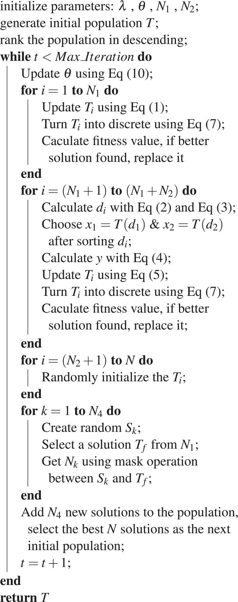
Algorithm 1: Pseudo-code of the BTGA.
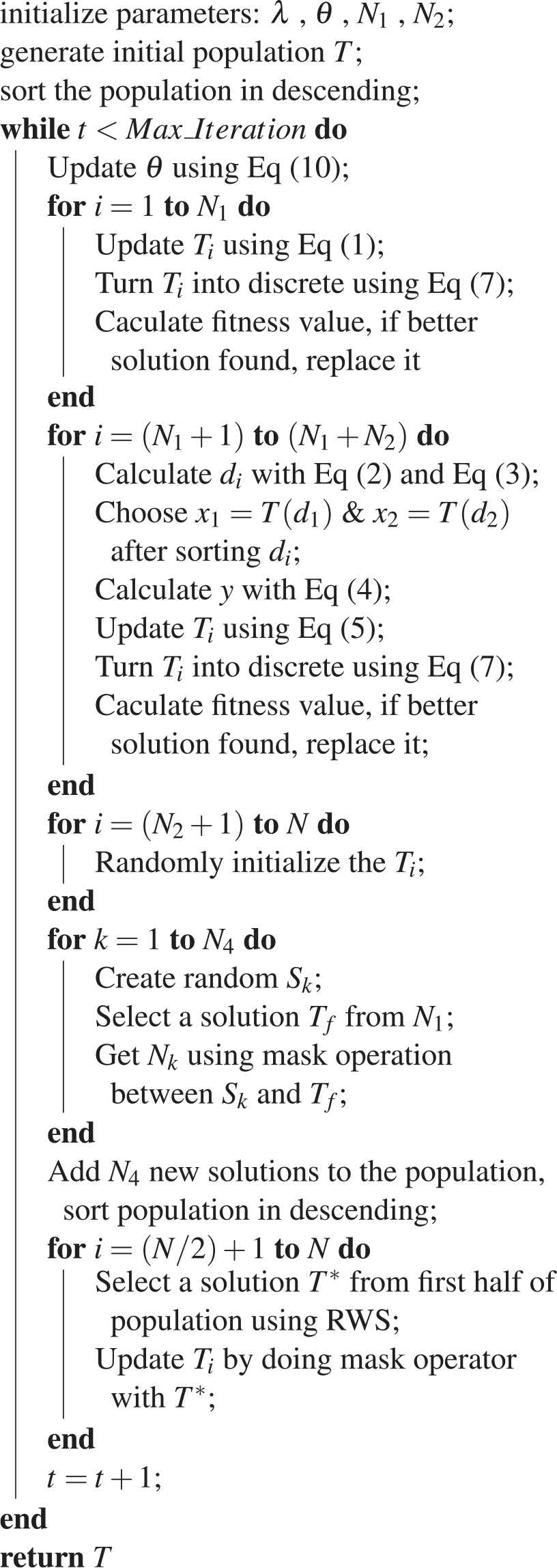
After selecting a solution from the first half of the population by using the RWS operator, it is used to reposition a solution from the second half by utilizing the mask operator. The overall pseudo-code of the iTGA is detailed in Algorithm 2.
Algorithm 2: Pseudo-code of the iTGA.
4. EXPERIMENTAL RESULTS AND DISCUSSIONS
In this section, fifteen feature selection benchmark datasets from the UCI [38] machine learning repository are selected to evaluate the efficiency of the proposed BTGA and iTGA. Table 1 gives a brief description of these datasets. These datasets are chosen to have various numbers of features, samples and classes as representatives of different kinds of problems, that can well exam the searchability of the algorithm in dealing with feature selection problems. For each dataset, the instances are randomly divided into two parts before each test, where 80% of the instances in the dataset is used for training and the remaining instances is utilized for testing. The commonly utilized K-nearest neighbor (KNN) learning algorithm is employed in the experiment to assess the candidate feature subsets. The experiment results in this research are conducted using MATLAB R2016a on a personal computer with Intel Core i5-2320 3.00GHz and 6GB RAM.
| No | Dataset | Features | Instances | Classes | Data area |
|---|---|---|---|---|---|
| 1 | Breastcancer | 9 | 699 | 2 | Biology |
| 2 | HeartEW | 13 | 270 | 2 | Biology |
| 3 | WineEW | 13 | 178 | 3 | Chemistry |
| 4 | Zoo | 16 | 101 | 7 | Artificial |
| 5 | CongressEW | 16 | 435 | 2 | Politics |
| 6 | Lymphography | 18 | 148 | 4 | Biology |
| 7 | SpectEW | 22 | 267 | 2 | Biology |
| 8 | BreastEW | 30 | 569 | 2 | Biology |
| 9 | IonosphereEW | 34 | 351 | 2 | Electromagnetic |
| 10 | Waveform | 40 | 5000 | 3 | Physics |
| 11 | SonarEW | 60 | 208 | 2 | Biology |
| 12 | Clean1 | 166 | 476 | 2 | Biology |
| 13 | Semeion | 265 | 1593 | 10 | Biology |
| 14 | Colon | 2000 | 62 | 2 | Biology |
| 15 | Leukemia | 7129 | 72 | 2 | Biology |
Used datasets.
In this paper, the number of search agents (
4.1. Comparison between Proposed Methods
In this part, convergence and the quality of the results of the proposed approaches are thoroughly evaluated and compared to investigate the influence of EPD strategy and RWS scheme on the proposed variants. For the sake of comparison, the results obtained from BTGA and iTGA are compared together in one table. Table 2 shows the attained fitness value, classification accuracy and the number of selected features and standard deviation (Std) results for BTGA approach versus iTGA.
| Fitness Value |
Classification Accuracy |
Selected Features |
Full |
||||||||||
|---|---|---|---|---|---|---|---|---|---|---|---|---|---|
| Datasets | BTGA |
iTGA |
BTGA |
iTGA |
BTGA |
iTGA |
KNN |
||||||
| Avg | Std | Avg | Std | Avg | Std | Avg | Std | Avg | Std | Avg | Std | ||
| Breastcancer | 0.022 | 0.010 | 0.020 | 0.010 | 0.982 | 0.010 | 0.984 | 0.010 | 4.166 | 1.116 | 4.3 | 0.876 | 0.9714 |
| HeartEW | 0.130 | 0.043 | 0.126 | 0.022 | 0.872 | 0.044 | 0.877 | 0.022 | 5.366 | 0.964 | 5.266 | 0.868 | 0.6704 |
| WineEW | 0.022 | 0.015 | 0.019 | 0.020 | 0.981 | 0.015 | 0.985 | 0.020 | 5.2 | 1.126 | 5.1 | 0.758 | 0.6910 |
| Zoo | 0.013 | 0.029 | 0.010 | 0.027 | 0.989 | 0.029 | 0.993 | 0.027 | 5.566 | 1.478 | 6.1 | 1.322 | 0.8812 |
| CongressEW | 0.021 | 0.011 | 0.020 | 0.014 | 0.982 | 0.011 | 0.983 | 0.014 | 6.3 | 1.600 | 6.733 | 1.460 | 0.9333 |
| Lymphography | 0.083 | 0.042 | 0.081 | 0.046 | 0.921 | 0.043 | 0.923 | 0.046 | 9.166 | 1.620 | 8.333 | 1.561 | 0.7703 |
| SpectEW | 0.106 | 0.032 | 0.100 | 0.041 | 0.897 | 0.039 | 0.903 | 0.041 | 10.833 | 1.795 | 10 | 1.485 | 0.7940 |
| BreastEW | 0.047 | 0.013 | 0.038 | 0.015 | 0.955 | 0.014 | 0.965 | 0.015 | 11.9 | 2.139 | 12.266 | 1.229 | 0.9279 |
| IonosphereEW | 0.092 | 0.027 | 0.083 | 0.034 | 0.910 | 0.024 | 0.920 | 0.034 | 15.166 | 2.865 | 15.633 | 1.884 | 0.8348 |
| Waveform | 0.170 | 0.007 | 0.167 | 0.008 | 0.834 | 0.007 | 0.838 | 0.007 | 29.133 | 3.936 | 28.2 | 3.977 | 0.8104 |
| SonarEW | 0.067 | 0.040 | 0.062 | 0.040 | 0.936 | 0.040 | 0.942 | 0.041 | 27.133 | 4.454 | 28.8 | 3.294 | 0.8125 |
| Clean1 | 0.060 | 0.021 | 0.058 | 0.018 | 0.944 | 0.022 | 0.946 | 0.018 | 91.733 | 12.025 | 89.933 | 7.338 | 0.8782 |
| Semeion | 0.021 | 0.006 | 0.022 | 0.009 | 0.984 | 0.006 | 0.984 | 0.009 | 130.733 | 20.631 | 139.166 | 12.253 | 0.9724 |
| Colon | 0.095 | 0.070 | 0.083 | 0.070 | 0.907 | 0.071 | 0.920 | 0.071 | 753.733 | 122.733 | 973.033 | 15.437 | 0.7903 |
| Leukemia | 0.014 | 0.030 | 0.013 | 0.022 | 0.988 | 0.030 | 0.991 | 0.023 | 2493.133 | 254.568 | 3484.066 | 13.310 | 0.9306 |
BTGA, binary tree growth algorithm; iTGA, improved tree growth algorithm.
The fitness value, classification accuracy, number of selected features of proposed methods.
It is obvious that in Table 2, iTGA can relatively outperform BTGA in terms of fitness value and classification accuracy over almost all datasets. The simple basic BTGA cannot expose higher accuracy than iTGA over all fifteen datasets. However, it can be seen from Table 2, either iTGA or BTGA have significantly improved the classification accuracy of using full feature set, especially in dealing with the HeartEW, WineEW, Zoo, Lymphography, SpectEW and Colon with an average increase of 16.5%. It is also can be revealed that iTGA can obtain superior classification accuracy compared to the basic optimizer in tacking the HeartEW, WineEW, Lymphography, SpectEW, Waveform and Clean1 datasets with fewer features. In tackling the Semeion, both BTGA and iTGA have obtained the same accuracy rate of 98.4%, while regarding the number of selected features in Table 2, BTGA with 130.733 selected features has outperformed iTGA. However, in terms of the Std of the selected features, iTGA is much lower than the basic optimizer.
It is obviously that the application of EPD strategy and RWS to the basic optimizer can bring significant performance improvement. The reason is that iTGA takes into account all individuals in the population during the evolution process, which help the algorithm to maintain the diversity of the population, and this make it has the ability to avoid local optima and find better solutions. In addition, the mask operator is utilized to relocate a solution from the poor half after selecting an individual with the RWS operator. The use of mask operator enabled iTGA to explore more virginal areas in the original feature space. The combination of these operators also improves the power of iTGA in balancing the exploration and exploitation as compared to the basic optimizer.
To expose the search process of BTGA and iTGA, Figures 2 and 3 show the iterative curves of the best solutions for all the datasets. As can be seen from Figures 2 and 3, feature selection does not mean that the fewer features the better. For example, in CongressEW of Figure 2 when seven features are selected at the 33th–54st iterations, the classification accuracy is 96.6%. However, the algorithm gets a feature subset with best classification accuracy 97.7% when eight features are selected. We can also see that feature selection is the process of continuously removing irrelevant and redundant features, and this can be well verified in the example of HeartEW in Figure 2.
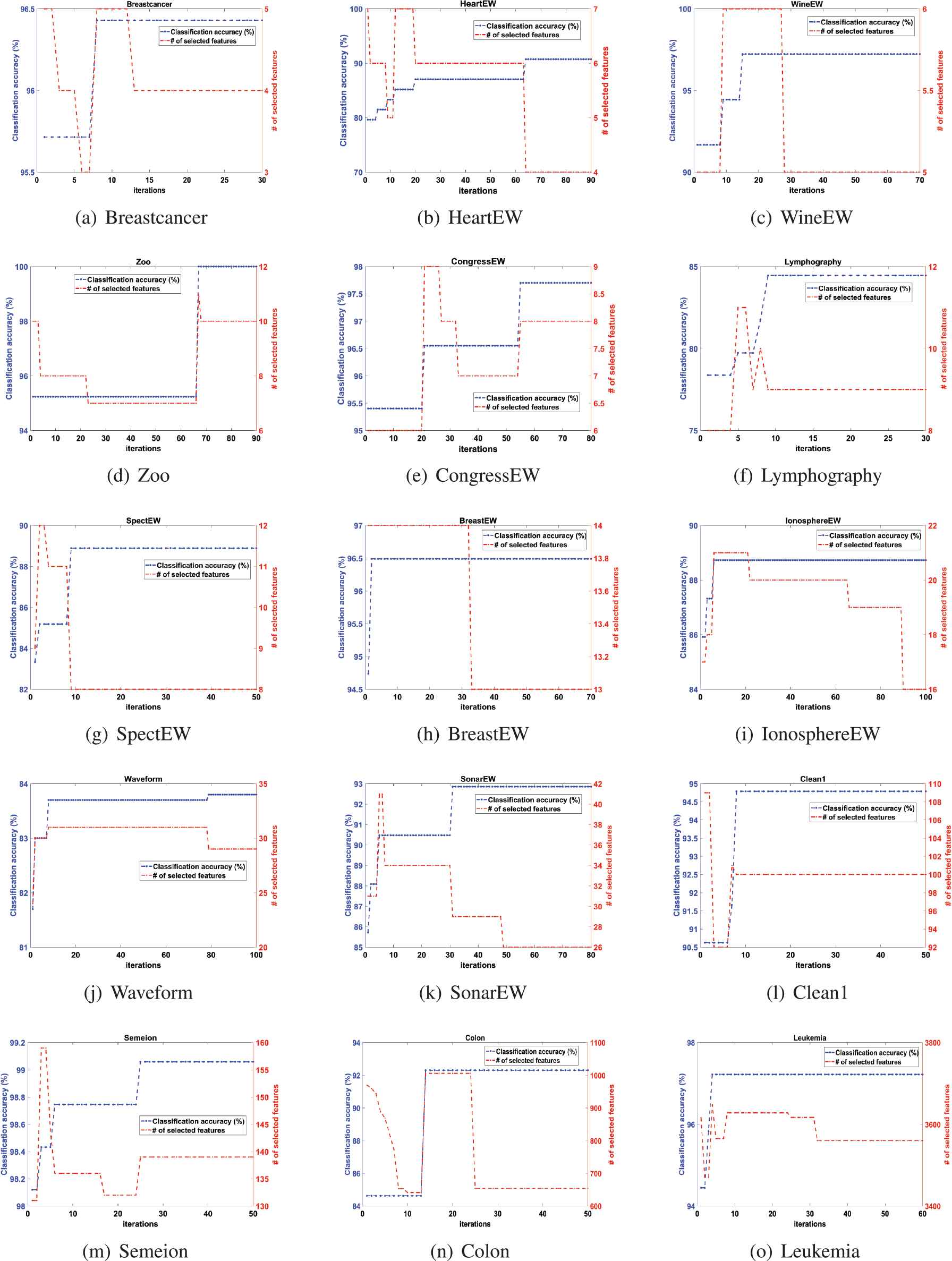
The iterative curves of solutions using binary tree growth algorithm (BTGA).
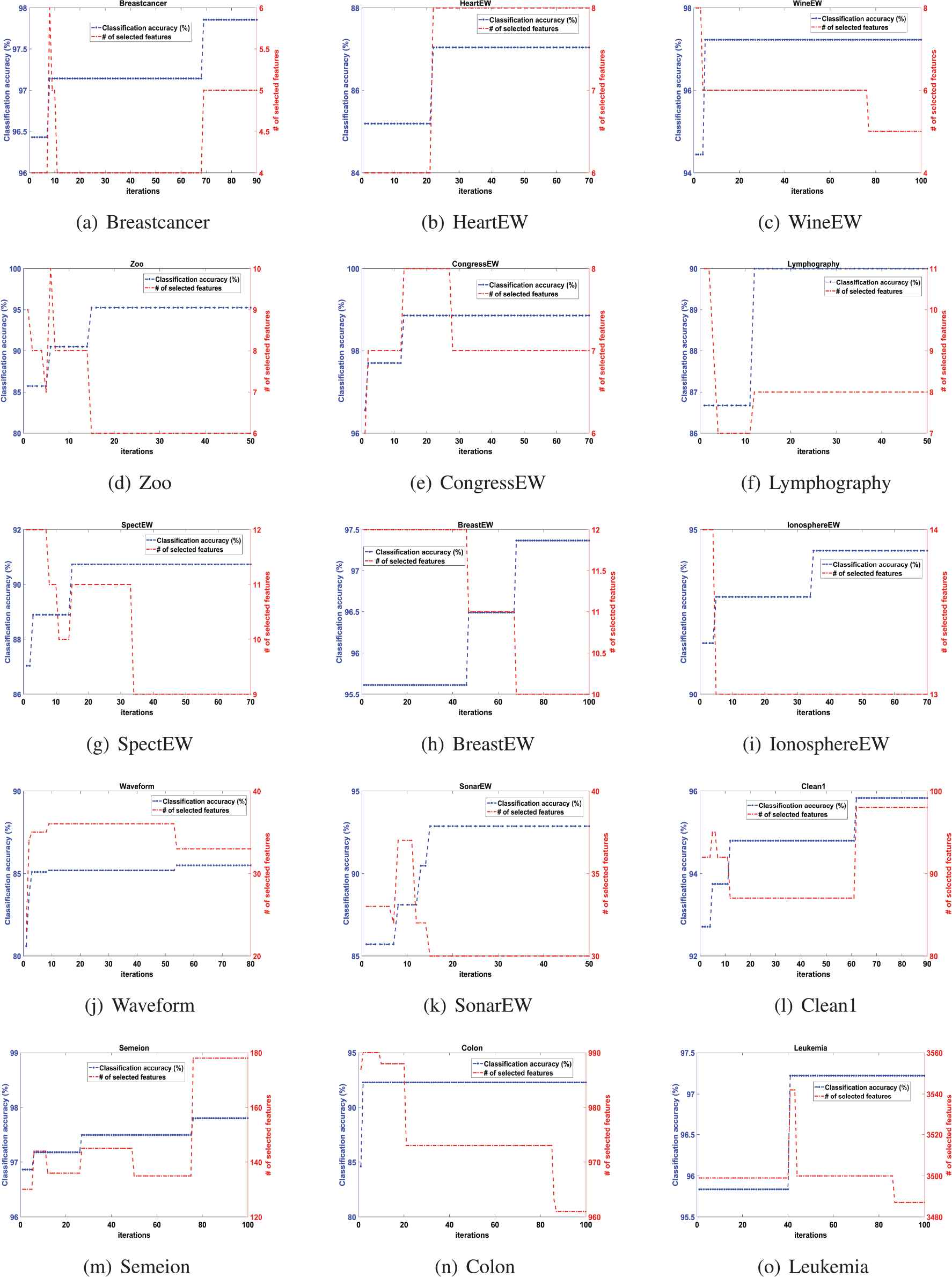
The iterative curves of solutions using improved tree growth algorithm (iTGA).
In dealing with HeartEW, the classification accuracy keeps rising, while the number of selected features maintains a decreasing trend. When seven features are selected at the 11th–20st iterations, the classification accuracy reaches 85%. After that, the redundant features are continuously removed, and the number of selected features is continuously reduced, but the classification accuracy is improved. Finally, the algorithm achieves 91% classification accuracy with only four features.
As can be seen from Figures 2 and 3, compared to iTGA, BTGA has been trapped in local optima in early steps of the exploration phase, for instance when tackling the Breastcancer, BreastEW, Clean1, IonosphereEW, Leukemia tasks. This reveals that improving the median of population using EPD strategy and RWS strategy may decrease the chance of iTGA to stagnated to local optima when searching the virginal regions of feature space. Therefore, it is shown that iTGA could find better solutions than BTGA in almost all instances. The trends of iTGA also show that the strategy of mask operator has enhanced the comprehensive learning of iTGA to balance the exploration and exploitation.
4.2. Compared with Other Metaheuristics
In this section, a comprehensive comparative experiment was implemented between our proposed methods and several state-of-the-art methods including the method based on binary gravity search algorithm (BGSA) [39]; the method based on binary bat algorithm (BBA) [40]; the method based on binary gray wolf optimization (BGWO) [41] and the method based on binary grasshopper optimization (BGOA) [25]. Without loss of generality, we used three general evaluation criteria to compare the performance of these algorithms. The general evaluation measures are shown below:
Classification accuracy: The average classification accuracy gained by using the selected features.
Number of selected features is the second comparison criterion.
The fitness value obtained from each approach is reported.
Wilcoxon's matched-pairs signed-ranks test [42] is used to detect whether the improved algorithm is significantly different from BTGA. Standard deviations of all proposed versions of measurements, datasets and algorithms are also provided. The results are presented in Tables 3–5. To evaluated the efficiency of these algorithms objectively, all of the results of BGOA, BGWO, BGSA and BBA were obtained directly from the reported literature [25].
| Dataset | BTGA |
iTGA |
BGSA |
BGOA |
BGWO |
BBA |
||||||
|---|---|---|---|---|---|---|---|---|---|---|---|---|
| Avg | StdDev | Avg | StdDev | Avg | StdDev | Avg | StdDev | Avg | StdDev | Avg | StdDev | |
| Breastcancer | 0.982 | 0.010 | 0.984 | 0.010 | 0.957 | 0.004 | 0.980 | 0.001 | 0.968 | 0.002 | 0.937 | 0.031 |
| HeartEW | 0.872 | 0.044 | 0.877 | 0.022 | 0.777 | 0.022 | 0.833 | 0.004 | 0.792 | 0.017 | 0.754 | 0.033 |
| WineEW | 0.981 | 0.015 | 0.985 | 0.020 | 0.951 | 0.015 | 0.989 | 0.000 | 0.960 | 0.012 | 0.919 | 0.052 |
| Zoo | 0.989 | 0.029 | 0.993 | 0.027 | 0.939 | 0.008 | 0.993 | 0.009 | 0.975 | 0.009 | 0.874 | 0.095 |
| CongressEW | 0.982 | 0.011 | 0.983 | 0.014 | 0.951 | 0.008 | 0.964 | 0.005 | 0.948 | 0.011 | 0.872 | 0.075 |
| Lymphography | 0.921 | 0.043 | 0.923 | 0.046 | 0.781 | 0.022 | 0.868 | 0.011 | 0.813 | 0.028 | 0.701 | 0.069 |
| SpectEW | 0.897 | 0.039 | 0.903 | 0.041 | 0.783 | 0.024 | 0.826 | 0.010 | 0.810 | 0.014 | 0.800 | 0.027 |
| BreastEW | 0.955 | 0.014 | 0.965 | 0.015 | 0.942 | 0.006 | 0.947 | 0.005 | 0.954 | 0.007 | 0.931 | 0.014 |
| IonosphereEW | 0.910 | 0.024 | 0.920 | 0.034 | 0.881 | 0.010 | 0.899 | 0.007 | 0.885 | 0.009 | 0.877 | 0.019 |
| Waveform | 0.834 | 0.007 | 0.838 | 0.007 | 0.695 | 0.014 | 0.737 | 0.003 | 0.723 | 0.007 | 0.669 | 0.033 |
| SonarEW | 0.936 | 0.040 | 0.942 | 0.041 | 0.888 | 0.015 | 0.912 | 0.009 | 0.836 | 0.016 | 0.844 | 0.036 |
| Clean1 | 0.944 | 0.022 | 0.946 | 0.018 | 0.898 | 0.011 | 0.863 | 0.004 | 0.908 | 0.006 | 0.826 | 0.021 |
| Semeion | 0.983 | 0.006 | 0.983 | 0.009 | 0.971 | 0.002 | 0.976 | 0.002 | 0.972 | 0.003 | 0.962 | 0.006 |
| Colon | 0.907 | 0.071 | 0.920 | 0.071 | 0.766 | 0.015 | 0.870 | 0.006 | 0.661 | 0.022 | 0.682 | 0.038 |
| Leukemia | 0.988 | 0.030 | 0.991 | 0.023 | 0.844 | 0.014 | 0.931 | 0.014 | 0.884 | 0.016 | 0.877 | 0.029 |
BBA, binary bat algorithm; BGOA, binary grasshopper optimization; BGSA, binary gravity search algorithm; BGWO, binary gray wolf optimization; BTGA, binary tree growth algorithm; iTGA, improved tree growth algorithm.
Classification accuracy results.
| Dataset | BTGA |
iTGA |
BGSA |
BGOA |
BGWO |
BBA |
||||||
|---|---|---|---|---|---|---|---|---|---|---|---|---|
| Avg | StdDev | Avg | StdDev | Avg | StdDev | Avg | StdDev | Avg | StdDev | Avg | StdDev | |
| Breastcancer | 4.166 | 1.116 | 4.3 | 0.876 | 6.067 | 1.143 | 5.000 | 0.000 | 7.100 | 1.447 | 3.667 | 1.373 |
| HeartEW | 5.366 | 0.964 | 5.266 | 0.868 | 6.833 | 1.315 | 8.400 | 1.037 | 8.167 | 2.001 | 5.900 | 1.647 |
| WineEW | 5.2 | 1.126 | 5.1 | 0.758 | 7.367 | 1.098 | 8.800 | 1.472 | 8.600 | 1.754 | 6.067 | 1.741 |
| Zoo | 5.566 | 1.478 | 6.1 | 1.322 | 8.167 | 1.177 | 9.167 | 1.967 | 10.367 | 2.484 | 6.567 | 2.501 |
| CongressEW | 6.3 | 1.600 | 6.733 | 1.460 | 6.767 | 2.402 | 5.767 | 2.012 | 7.300 | 2.136 | 6.233 | 2.063 |
| Lymphography | 9.166 | 1.620 | 8.333 | 1.561 | 9.167 | 1.895 | 10.633 | 1.217 | 11.100 | 1.971 | 7.800 | 2.203 |
| SpectEW | 10.833 | 1.795 | 10 | 1.485 | 9.533 | 2.300 | 11.100 | 3.044 | 12.633 | 2.442 | 7.967 | 2.282 |
| BreastEW | 11.9 | 2.139 | 12.266 | 1.229 | 16.567 | 2.979 | 17.333 | 2.440 | 19.000 | 4.307 | 12.400 | 2.762 |
| IonosphereEW | 15.166 | 2.865 | 15.633 | 1.884 | 15.400 | 2.513 | 16.400 | 3.701 | 19.233 | 5.015 | 13.400 | 2.594 |
| Waveform | 29.133 | 3.936 | 28.2 | 3.977 | 19.900 | 2.917 | 26.233 | 3.451 | 31.967 | 4.612 | 16.667 | 3.304 |
| SonarEW | 27.133 | 4.454 | 28.8 | 3.294 | 30.033 | 3.700 | 36.767 | 4.240 | 36.233 | 8.613 | 24.700 | 5.377 |
| Clean1 | 91.733 | 12.025 | 89.933 | 7.338 | 83.700 | 5.421 | 92.600 | 7.802 | 121.267 | 20.691 | 64.767 | 10.016 |
| Semeion | 130.733 | 20.631 | 139.166 | 12.253 | 133.533 | 7.422 | 157.033 | 11.485 | 200.100 | 31.022 | 107.033 | 10.947 |
| Colon | 753.733 | 122.733 | 973.033 | 15.437 | 995.833 | 20.021 | 1063.667 | 64.618 | 1042.100 | 126.721 | 827.500 | 55.371 |
| Leukemia | 2493.133 | 254.568 | 3484.066 | 13.310 | 3555.133 | 39.713 | 3768.800 | 224.842 | 3663.767 | 294.872 | 2860.000 | 247.642 |
BBA, binary bat algorithm; BGOA, binary grasshopper optimization; BGSA, binary gravity search algorithm; BGWO, binary gray wolf optimization; BTGA, binary tree growth algorithm; iTGA, improved tree growth algorithm.
Average number of selected features results.
| Dataset | BTGA |
iTGA |
BGSA |
BGOA |
BGWO |
BBA |
||||||
|---|---|---|---|---|---|---|---|---|---|---|---|---|
| Avg | StdDev | Avg | StdDev | Avg | StdDev | Avg | StdDev | Avg | StdDev | Avg | StdDev | |
| Breastcancer | 0.022 | 0.010 | 0.020 | 0.010 | 0.049 | 0.003 | 0.026 | 0.001 | 0.039 | 0.003 | 0.044 | 0.005 |
| HeartEW | 0.130 | 0.043 | 0.126 | 0.022 | 0.226 | 0.021 | 0.171 | 0.004 | 0.213 | 0.017 | 0.208 | 0.015 |
| WineEW | 0.022 | 0.015 | 0.019 | 0.020 | 0.054 | 0.015 | 0.018 | 0.001 | 0.047 | 0.012 | 0.036 | 0.013 |
| Zoo | 0.013 | 0.029 | 0.010 | 0.027 | 0.065 | 0.008 | 0.012 | 0.008 | 0.032 | 0.009 | 0.042 | 0.015 |
| CongressEW | 0.021 | 0.011 | 0.020 | 0.014 | 0.053 | 0.008 | 0.039 | 0.005 | 0.056 | 0.011 | 0.064 | 0.015 |
| Lymphography | 0.083 | 0.042 | 0.081 | 0.046 | 0.222 | 0.022 | 0.137 | 0.011 | 0.191 | 0.028 | 0.226 | 0.024 |
| SpectEW | 0.106 | 0.032 | 0.100 | 0.041 | 0.220 | 0.024 | 0.177 | 0.010 | 0.194 | 0.014 | 0.172 | 0.012 |
| BreastEW | 0.047 | 0.013 | 0.038 | 0.015 | 0.063 | 0.006 | 0.058 | 0.004 | 0.051 | 0.007 | 0.056 | 0.006 |
| IonosphereEW | 0.092 | 0.027 | 0.083 | 0.034 | 0.122 | 0.012 | 0.105 | 0.007 | 0.120 | 0.009 | 0.108 | 0.012 |
| Waveform | 0.170 | 0.007 | 0.167 | 0.008 | 0.307 | 0.014 | 0.267 | 0.003 | 0.283 | 0.007 | 0.304 | 0.014 |
| SonarEW | 0.067 | 0.040 | 0.062 | 0.040 | 0.116 | 0.015 | 0.094 | 0.008 | 0.169 | 0.016 | 0.110 | 0.021 |
| Clean1 | 0.060 | 0.021 | 0.058 | 0.018 | 0.106 | 0.010 | 0.141 | 0.004 | 0.099 | 0.006 | 0.156 | 0.013 |
| Semeion | 0.021 | 0.006 | 0.021 | 0.009 | 0.034 | 0.002 | 0.030 | 0.001 | 0.036 | 0.003 | 0.033 | 0.003 |
| Colon | 0.095 | 0.070 | 0.083 | 0.070 | 0.237 | 0.014 | 0.134 | 0.006 | 0.341 | 0.022 | 0.279 | 0.035 |
| Leukemia | 0.014 | 0.030 | 0.013 | 0.022 | 0.160 | 0.013 | 0.073 | 0.014 | 0.120 | 0.016 | 0.085 | 0.023 |
BBA, binary bat algorithm; BGOA, binary grasshopper optimization; BGSA, binary gravity search algorithm; BGWO, binary gray wolf optimization; BTGA, binary tree growth algorithm; iTGA, improved tree growth algorithm.
Fitness value results.
Table 3 presents the obtained average classification accuracy and related standard deviation results for the proposed algorithms versus other methods. Tables 4 and 5 also reflect the average selected features, fitness along with the related standard deviation for the compared algorithms. Note that the best results are highlighted in bold. In addition, Wilcoxon's matched-pairs signed-ranks test was applied to compare these algorithms over all the datasets. Tables 6 and 7 show the results of Wilcoxon's matched-pairs signed-ranks test for the classification accuracy and fitness value in Tables 3 and 5.
| iTGA vs | R+ | R− | P value |
|---|---|---|---|
| BTGA | 120 | 0 | 1.2207e-04 |
| BGSA | 120 | 0 | 6.1035e-5 |
| BGOA | 117 | 3 | 0.0018 |
| BGWO | 120 | 0 | 6.1035e-5 |
| BBA | 120 | 0 | 6.1035e-5 |
BBA, binary bat algorithm; BGOA, binary grasshopper optimization; BGSA, binary gravity search algorithm; BGWO, binary gray wolf optimization; BTGA, binary tree growth algorithm; iTGA, improved tree growth algorithm.
Wilcoxon's matched-pairs test on classification accuracy.
| iTGA vs | R+ | R− | P value |
|---|---|---|---|
| BTGA | 111 | 9 | 1.2207e-04 |
| BGSA | 120 | 0 | 6.1035e-05 |
| BGOA | 119 | 1 | 9.7656e-04 |
| BGWO | 120 | 0 | 6.1035e-05 |
| BBA | 120 | 0 | 6.1035e-05 |
BBA, binary bat algorithm; BGOA, binary grasshopper optimization; BGSA, binary gravity search algorithm; BGWO, binary gray wolf optimization; BTGA, binary tree growth algorithm; iTGA, improved tree growth algorithm.
Wilcoxon's matched-pairs test on fitness value.
Note that the computational complexity of GOA and bat algorithm (BA) is of
From Table 3, it can be observed that the good performance of iTGA approach compared to other methods. iTGA outperform all contestants on fourteen datasets. BGOA also outperform others two problems: WineEW and Zoo. In tackling the Zoo dataset, both BGOA and iTGA achieve the same classification accuracy 99.3%, while based on the number of selected features in Table 4, iTGA with 6.1 selected features outperform BGOA. Compared with BGWO, iTGA can provide better results on all issues. In tackling all fifteen datasets, the classification accuracy of iTGA have increased in the range of 1.1% (Semeion) to 25.9% (Colon) in comparison with BGWO. At the same time, iTGA outperformed BGSA and BBA on all datasets as well. This results demonstrate that our proposed method has the ability to explore the solution space and find the best feature subset that produces higher classification accuracy.
The main reason for increased classification accuracy of the proposed method is that iTGA using the EPD strategy to relocate the poor solutions around the better ones. During this process, the RWS mechanism help iTGA to keep the diversity of population by giving the poor solutions a chance to mutated and crossover with better ones. After that, the population restores a stable balance state between exploration and exploitation. In this way, they can escape from the case of stagnation to local optima using the stochastic nature behind the utilized strategy.
From the results in Table 4, it can be seen that BBA is superior to other algorithms on eight datasets. BTGA and iTGA attained the second and the third. For HeartEW and WineEW dataset, it is found that iTGA can provide the best results.
From the results in Table 5, it can be seen that the proposed approach can outperform other methods and obtain the best fitness value in tackling fourteen datasets. Furthermore, our proposed approach attains better costs compared to BGOA on 86.6% of the datasets, and outperforms other algorithms on all datasets. The reason is that the EPD strategy and RWS mechanism assist the proposed method to keep the diversity of population and the use of mask operator also enhances the exploitative ability of the algorithm. All of these make iTGA has the ability of keeping a stable balance between the exploration and exploitation during the optimization process.
Wilcoxon's matched-pairs signed-ranks test [42] was applied to compare these algorithms on all the datasets. This test calculates the performance differences of two algorithms and ranks them based on their magnitudes. Rankings are aggregated according to their sign R+ for iTGA and R- for the other method. Finally, we calculate the probability that supports the null-hypothesis, the p-value, which assumes that the performance of these algorithms is equivalent. Tables 6 and 7 present the results of the Wilcoxon test for each criterion.
From the results in Tables 6 and 7, it can be seen that none of the contrast algorithm outperforms iTGA. On the contrary, iTGA often provides statistically better results. Based on the results obtained, we can conclude that the EPD strategy and RWS mechanism have improved the balance between exploration and exploitation. Therefore, iTGA can overcome the drawback of being trapped into local optima.
4.3. Compared with Filter-Based Methods
In this section, the classification accuracy of iTGA is compared with five well-known filter-based feature selection methods: fast correlation-based filters (FCBF) [43], correlation-based feature selection (CFS) [10], F-score [8], IG [7] and Spectrum [44]. These methods are selected from two different categories: univariate and multivariate methods. The F-Score, IG and Spectrum are from univariate filter-based methods that do not consider the dependence of features in the evaluation criterion. The CFS and FCBF come from the multivariate filter-based categories, which the dependencies between features is considered in the evaluation of the correlation of features.
The reason why these methods are compared is that they have different strategies to utilize the class label of the training datasets to accomplish the analysis of feature relevance. The supervised methods include FCBF, CFS, IG and F-score are able to use class tags, while the unsupervised approaches such as Spectrum cannot utilize class tags for analyzing the features. Table 8 illustrated the results of average classification accuracy after 30 runs using these filter-based methods and iTGA.
| Dataset | CFS | FCBF | F-score | IG | Spectrum | iTGA |
|---|---|---|---|---|---|---|
| Breastcancer | 0.957 | 0.986 | 0.979 | 0.957 | 0.957 | 0.984 |
| HeartEW | 0.648 | 0.648 | 0.759 | 0.759 | 0.796 | 0.877 |
| WineEW | 0.778 | 0.889 | 0.861 | 0.889 | 0.889 | 0.985 |
| Zoo | 0.800 | 0.900 | 0.650 | 0.850 | 0.600 | 0.993 |
| CongressEW | 0.793 | 0.793 | 0.908 | 0.828 | 0.828 | 0.983 |
| Lymphography | 0.500 | 0.567 | 0.667 | 0.667 | 0.767 | 0.923 |
| SpectEW | 0.736 | 0.774 | 0.793 | 0.793 | 0.736 | 0.903 |
| BreastEW | 0.825 | 0.798 | 0.930 | 0.930 | 0.772 | 0.965 |
| IonosphereEW | 0.857 | 0.857 | 0.729 | 0.800 | 0.829 | 0.920 |
| Waveform | 0.620 | 0.710 | 0.662 | 0.662 | 0.292 | 0.838 |
| SonarEW | 0.310 | 0.214 | 0.048 | 0.191 | 0.048 | 0.942 |
| Clean1 | 0.716 | 0.642 | 0.632 | 0.547 | 0.611 | 0.946 |
| Semeion | 0.875 | 0.875 | 0.875 | 0.868 | 0.875 | 0.983 |
| Colon | 0.750 | 0.667 | 0.667 | 0.667 | 0.500 | 0.920 |
| Leukemia | 0.929 | 0.857 | 0.980 | 0.980 | 0.357 | 0.991 |
CFS, correlation-based feature selection; FCBF, fast correlation-based filters; IG, information gain; iTGA, improved tree growth algorithm.
Classification accuracy results of filter-based methods and iTGA.
From the results in Table 8, it is clear that our proposed algorithm can outperform other filter-based methods on fourteen datasets, while the FCBF algorithm provided the best result for Breastcancer dataset. iTGA outperform the supervised univariate feature selection methods include F-Score and IG, the supervised multivariate feature selection method such as CFS and FCBF, and the unsupervised Spectrum method. The experimental results show that the proposed method can effectively mine the feature space, find the optimal reduction, and improve the classification accuracy. The results also prove that the wrapper-based feature selection methods can provide better solutions than filter-based approaches because they can use both class labels and correlations during the selection of feature subsets.
5. CONCLUSIONS
Feature selection plays a substantial role in data preprocessing that speeds up the model building process and improves algorithm performance by excluding the redundant and irrelevant features. The wrapper-based feature selection methods suffered from high computational cost of selecting the appropriate feature subset from a high-dimensional feature space. Therefore, the metaheuristics, which are well-regarded for their powerful global search ability, provide a new way to solve feature selection problems.
TGA is a recent proposed population-based metaheuristic, which shows great power of search ability in solving optimization of continuous problems. However, TGA cannot be directly applied to feature selection problems. Also, we find that its efficiency still leave room for improvement. For this reason, in this paper, a novel iTGA is proposed to tackle the feature selection problems. First, we presented a new binarization method to transform the algorithm from continuous to discrete version to solve the problem of feature selection. Second, a linearly increasing parameter tuning mechanism is proposed to tune the parameter in TGA. Third, TGA was equipped with EPD strategy to improve the search ability of TGA in solving feature selection problems. Fourth, fifteen well-known UCI datasets were selected to asses and compare the performance of our method with other metaheuristics and some filter-based feature selection methods. Three criteria were reported to evaluate each approach: classification accuracy, fitness value, number of selected features.
We believe that the use of linearly increasing parameter tuning mechanism and EPD strategy improves the search ability of the algorithm and prevent algorithm from stagnating into local optima, so as to obtain better results. The result of comparative experiments also verify the superiority of iTGA compared with other state-of-the-art methods.
CONFLICT OF INTEREST
The authors declare no conflicts of interest.
AUTHORS' CONTRIBUTIONS
Changkang Zhong and Yu Chen implemented all the experiments and were in charge of writing. Changkang Zhong conceived the idea and developed the main algorithm. Jian Peng checked the correctness of the theory and the writing. Notice that Changkang Zhong and Yu Chen contributed equally to this work.
ACKNOWLEDGMENTS
We would like to thank Armin Cheraghalipour, the author of TGA, for providing us the source code of TGA and discussing with us the details about TGA. This work is supported by the National Key Research and Development Program of China (Grant No.2017YFB0202403), the sub-project of the Special Fund for Key Program of Science and Technology of Sichuan Province (Grant No.2017GZDZX0003), Zigong School-Science and Technology Cooperation Special Fund (Grant No.2018CDZG-15) and Sichuan Key Research and Development Program (Grant No.2019KJT0015-2018GZ0098, Grant No.2018GZDZX0010).
REFERENCES
Cite this article
TY  - JOUR
AU  - Changkang Zhong
AU  - Yu Chen
AU  - Jian Peng
PY  - 2020
DA  - 2020/02/26
TI  - Feature Selection Based on a Novel Improved Tree Growth Algorithm
JO  - International Journal of Computational Intelligence Systems
SP  - 247
EP  - 258
VL  - 13
IS  - 1
SN  - 1875-6883
UR  - https://doi.org/10.2991/ijcis.d.200219.001
DO  - 10.2991/ijcis.d.200219.001
ID  - Zhong2020
ER  -