
Using Market Sentiment Analysis and Genetic Algorithm-Based Least Squares Support Vector Regression to Predict Gold Prices
- DOI
- 10.2991/ijcis.d.200214.002How to use a DOI?
- Keywords
- Gold price prediction; Text mining; Opinion score; Genetic algorithms; Least square support vector regression
- Abstract
Gold price prediction has long been a crucial and challenging research topic for gold investors. In conventional models, most scholars have used the historical gold price or economic indicators to forecast gold prices. The gold prices depend mainly on confidence in the current market. To reduce the time delay of economic indicators in this study, the daily online global gold news undergoes a text mining approach. An opinion score is generated by ascertaining the opinion polarity and words in the daily gold news. The opinion score represents the current market trends and used as an input predictor in the forecasting model. Subsequently, the least square support vector regression (LSSVR) that is optimized by the genetic algorithm (GA) is employed to train and predict the future gold price. The mean absolute percentage error (MAPE) is adopted to evaluate the model performance. This study is the first to use the opinion score through text mining as an input predictor to GA-LSSVR in forecasting gold prices. The experiment results demonstrate that the input predictor, opinion score, can improve the predicting ability of GA-LSSVR model in terms of MAPE.
- Copyright
- © 2020 The Authors. Published by Atlantis Press SARL.
- Open Access
- This is an open access article distributed under the CC BY-NC 4.0 license (http://creativecommons.org/licenses/by-nc/4.0/).
1. INTRODUCTION
Gold is a commodity that can be used as an investment and hedging tool, and numerous investment products are traded in the global market. Many people use gold to preserve wealth from generation to generation. Gold has been traded actively on the international market for a long time. Over the past 20 years, the investment industry has undergone rapid and far-reaching changes. The subprime mortgage crisis in the United States led to the 2007–2012 global financial crisis, which has caused many economic problems and the price of financial products to be unpredictable. However, gold prices have continued to fall as the global economic recovery led to substantially decreased demand for gold as a hedge against inflation. Thus, to stimulate retail investors to purchase physical gold, gold prices rebounded from a low. The gold price depends mainly on confidence in the current market. Therefore, establishing an accurate gold price forecasting model is vital to help the investor to gain profit and reduce investment risk. Besides, gold can smooth inflation fluctuations; hence, governments use gold as a price controlling and monetary policy lever [1]. Accordingly, forecasting gold price has become very important.
Many gold price forecasting models have been proposed to continue improving forecasting performances. Guha and Bandyopadhyay [2] used Autoregressive Integrated Moving Average (ARIMA) model to forecast Gold Price. The statistical model often fails due to market fluctuations, and can't forecast satisfactorily when strong nonlinear and nonstationary signals are involved. Therefore, most of the forecasting work focuses on time series prediction with various Artificial Intelligence models, such as artificial neural networks (ANN). Due to its superior nonlinear processing capability and fault-tolerant ability, different ANN models have been widely applied to improve the performance of gold price forecasting. The hybrid model of Genetic Algorithm and Neural network (GA-BP) has been proposed by Chunmei [3], and the experimental results indicated that the prediction model yields acceptable results. The radial basis function (RBF) neural network has been presented by Hussein et al. [4]. However, the result obtained is not promising. Multi-layered feed forward (MLFF) and group method of data handling (GMDH) neural network have been presented by Varahrami [5]. The experimental results indicated that the effect of GMDH is better than MLFF. Adaptive network-based fuzzy inference system (ANFIS) was used by Yazdani-Chamzini et al. [6]. The results showed that the ANFIS model outperforms ANN and ARIMA model. BAT-neural network (BNN) has been proposed by Hafezi et al. [7]. The results showed that the BNN model outperforms other benchmark models such as ARIMA, ANN, and ANFIS. However, the practicability of these proposed ANN models is affected due to several weaknesses, such as time-consuming, slow convergence velocity, trapping into local optimal solution easily [8–12], and challenging to determine suitable network structure [13].
Therefore, ANN is not recommended to be an excellent forecasting tool [14]. So, there are a lot of machine learning algorithms to take its place. Unlike ANN models, the support vector regression (SVR) and least square support vector regression (LSSVR) can solve nonlinear forecasting problems, avoid over-learning, local minima, and dimension disaster problems [12]. Artificial Bee Colony (ABC)-LSSVR has been proposed by Mustaffa and Yusof [15]. Compared with Back Propagation Neural Network (BPNN), the proposed approach shows that the combination of LSSVR and ABC leads to better performance. SVR was used by Dubey to forecast Gold price [16]. It was observed that the models obtained using SVR outperformed the ANFIS models. SVR and LSSVR have become two promising forecasting methodologies.
However, there are still some problems with the above methods. More importantly, they have neglected other source of information such as mass media that will significantly affect the behavior of investors. In the 1990s, when the Internet became widespread, news spread across the world instantaneously. Investors were easily influenced by international news on financial commodities and changed their investment decisions. Recently, some scholars use text mining technology to provide references for investors, such as stock price forecasting [17], oil price forecasting, foreign exchange forecasting [18]. Chen et al. [19] have integrated the ANN and text mining to forecast gold futures prices. This study only identified nonquantitative factors by text mining to help explain the trend and volatility of future gold prices. However, the research on gold price prediction has been rarely seen.
Text mining is the process of retrieving useful information from textual data. Recently, sentiment analysis from text mining, also called opinion mining, is used to analyze opinion polarities for a product or topic, such as positive, negative, or neutral. In other words, according to the research needs, the polarity indicator of the document content is defined, and the polarity indicator score is calculated as the opinion score, a quantitative variable transferred from nonquantifiable factors, which is one predictor used in the prediction model. Opinion scores represent the current market trends. To date, few scholars apply the opinion score of text mining technology to predict the gold price.
However, using investors' expectations caused by news alone is inadequate. Therefore, this research will combine the opinion scores obtained from the news release and conventional variables used frequently by researchers to enhance the predictability of the gold prices forecasting. Conventionally, gold price forecasting studies consider only gold spot or gold futures as variables [3–5,20–22]. However, some scholars [15,19,23,24] believe that additional factors are also associated with gold price fluctuation, such as stock index, U.S. dollar exchange rate, and crude oil prices. Therefore, this study integrates the variables frequently used in the literature into our prediction model, including the prices of precious metals (e.g., gold, silver, platinum, and palladium) and economic indicators (i.e., the federal funds rate, U.S. dollar index, crude oil prices, and U.S. S&P 500 index). Because the selected input variables can influence forecasting accuracy, identifying the most critical to establishing the forecasting model is necessary to obtain more accurate forecasting results. Therefore, in this study, the opinion scores together with those above frequently used conventional variables undergo correlation analysis to select the optimal combination of predictors to predict gold prices.
On the other hand, SVR and LSSVR have become two promising forecasting tools, as mentioned above. SVR may be seen to yield impressive results and has been a widely used and effective forecasting model in recent years [12]. However, the major drawback of SVR is low speed in the training phase [25]. An alternative proposed method, LSSVR introduced by Brabanter, Brabanter, Suykens, and Moor [27], is a more computationally efficient nonlinear function estimator modified from the SVR. LSSVR can improve the training speed of solving the problem by transforming the quadratic programming problem of SVR into solving the problem of linear equations [28]. Hence, LSSVR has demonstrated superior performances [29–31] and has been applied to many forecasting areas, including reliability analysis [32], pH indications prediction [33], crashworthiness optimization problems [34], financial prediction [15], foreign exchange rate forecasting [35], revenue forecasting [36], tourism demand forecasting [29], beta systematic risk forecasting [37], crude oil price forecasting [38,39], robust system identification with outliers [40], solar irradiance forecasting [41], wind speed prediction [42], and so on. Therefore, this paper tends to introduce this powerful forecasting technique of LSSVR to perform prediction for gold prices. However, the prerequisite for LSSVR to achieve more accurate results is to identify two appropriate user-defined hyper-parameters, namely regularization parameter (γ) and kernel parameter (σ2), which play key roles in constructing a highly accurate regression model with favorable generalization performance.
Yusof and Mustaffa [31] have reviewed existing works and learned that optimizing the hyper-parameters of LSSVR is best implemented using the evolutionary algorithms (EA). Categorized under EA group, GA is the most prominent and widely used technique as compared with other techniques within the same domain [43]. GA has a strong global search capability and can rapidly obtain the optimal solution. Thus, GA has been widely used to search for effective parameter combinations for LSSVR [33,37,38,43]. In the GA–LSSVR model, the regularization parameter and kernel parameter of LSSVR are dynamically optimized by implementing the evolutionary process with a randomly generated initial population of chromosomes, following which the LSSVR model performs the prediction task using these optimal values.
To the best of our knowledge, this study is the first research to use opinion score from text mining as input predictor to forecast in gold price prediction. This work has the objective of verifying the effectiveness of opinion scores used in developed GA-LSSVR model for forecasting gold prices. Comparisons of the results with those obtained using various predictors indicate the potential of the proposed approach, which can provide comparable or more accurate gold price predictions. The opinion score can improve gold price predictions, and thus, it can significantly affect gold price forecasting.
The remainder of this paper is organized as follows: Section 2 introduces the methodologies; Section 3 presents and discusses the experimental results, and Section 4 concludes the paper.
2. METHODOLOGY
2.1. Least Square Support Vector Regression
The LSSVR is a more computationally efficient nonlinear function estimator modified from the SVR [29,38,46–51]. LSSVR uses the least squares loss function instead of the ε-insensitive loss function. The solution follows from a linear Karush–Kuhn–Tucker (KKT) system instead of a computationally hard quadratic programming (QP) problem [27]. We can obtain the LSSVR regression model by solving the following optimization problem [37]:
Minimize
After w and e are eliminated, the (KKT) system is obtained as follows:
2.2. Least Squares Support Regression Parameters Optimization Method Based on GA
In the GA-LSSVR model, regularization parameter (γ) and kernel parameter (σ2) of LSSVR are dynamically optimized by implementing the evolutionary process with a randomly generated initial population of chromosomes, and the LSSVR model then performs the prediction task using two candidate values. Our approach simultaneously determines the optimal parameter values for optimizing the LSSVR model. Figure 1 illustrates the process of the GA-LSSVR model.
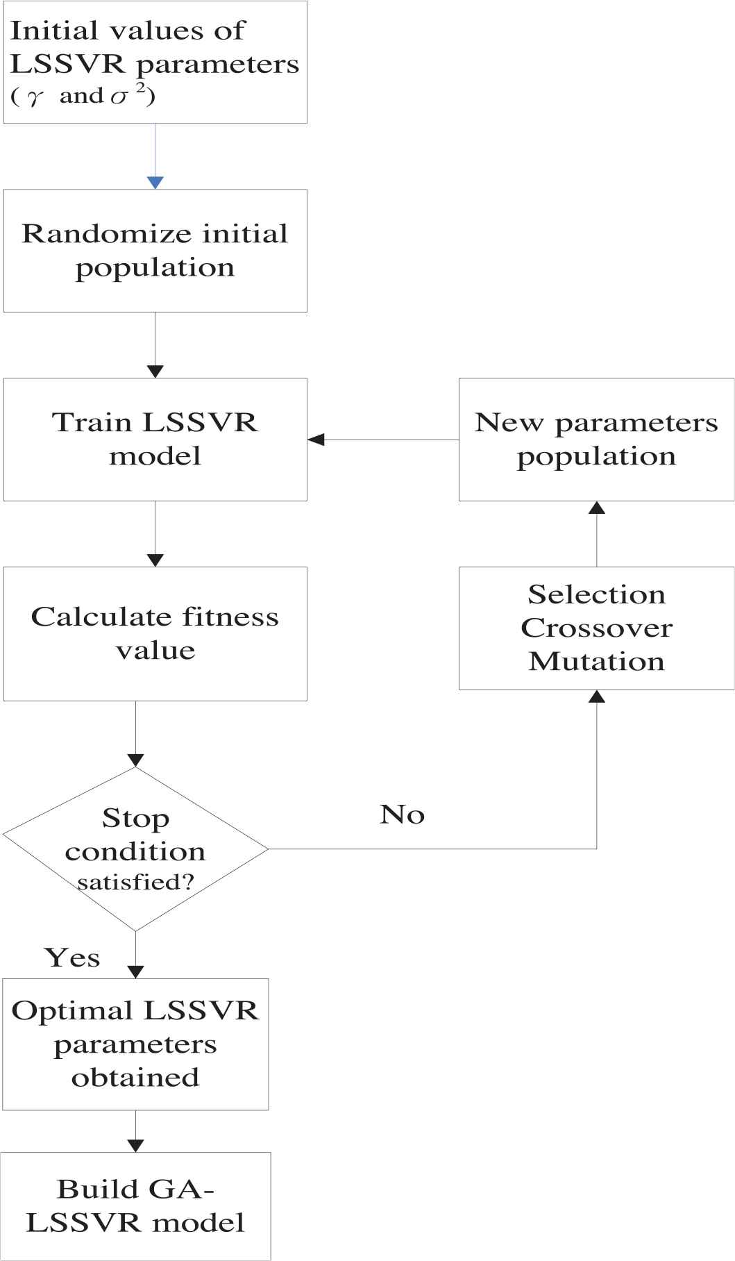
Genetic algorithm-least square support vector regression (GA-LSSVR) model.
Details of the proposed GA-LSSVR model are presented as follows:
Step 1. Chromosome representations. Both LSSVR's hyper-parameters, γ and σ2, are directly coded to generate the chromosome by using real-value GAs. Hence, chromosome Y can be represented as Y = [c1, c2], where c1 and c2 denote γ and σ2, respectively. In this model, the initial population is composed of 100 random chromosomes.
Step 2. Fitness function. To obtain the optimal LSSVR's parameters, a fitness function must be specified in advance for assessing the performance of each chromosome. This study employed the mean absolute percentage error (MAPE) given in Equation (6) as the fitness value for evaluating the modeling accuracy of the GA-LSSVR model.
Step 3. Genetic operators. Genetic operator includes selection, crossover, and mutation to generate the offspring of the existing population. The tournament selection strategy [53] is adopted to select chromosomes for reproduction, and elitist chromosomes are reserved. Once a pair of chromosomes has been selected for the crossover, one or more randomly selected positions are assigned into the to-be-crossed chromosomes. The newly-crossed chromosomes then combine with the rest of the chromosomes to generate a new population. The mutation operation follows the crossover to determine whether or not a chromosome should mutate in the next generation. The standard uniform mutation method [33] was used in this model.
Step 4. Stopping criteria. The process is repeated, as shown in Figure 1 until the generation number is equal to 1000 with MAPE convergence. When the termination condition is satisfied, the optimal combination of the hyper-parameters, γ and σ2, is used to construct the GA-LSSVR model.
2.3. Evaluating the Performance Index
Several measurement indicators have been proposed and employed to assess the prediction accuracy of models such as MAPE and mean-square error (MSE) and so on. The most frequently used measure is the MAPE [54]. A significant advantage of this measure is that it does not depend on the magnitudes of the forecast variables. Witt and Witt [55] suggested that MAPE is the most appropriate error measure for evaluating forecasting performance. In this study, the MAPE is used to evaluate the forecasting accuracy through cross-sectional analysis.
2.4. Text Preprocessing
cnYES is the portal to the financial industry, providing the richest, the most professional, and the most diversified global financial information and news in Chinese. The gold news provided by cnYES news can be searched by date, fewer noise data, and convenience. Therefore, this study chooses cnYES news as its text mining data source. The text preprocessing steps are as follows:
Web crawling and parsing: A web crawler program is developed to crawl gold news from cnYES, including date, title, and content.
Word segmentation: A Chinese knowledge information process (CKIP, http://ckip.iis.sinica.edu.tw/CKIP//index/htm) is used for word segmentation.
Part-of-speech tagging: CKIP is used for part-of-speech tagging. An example of word segmentation and part-of-speech tagging is provided in Table 1.
Stop word filtering: Stop words, such as pronouns, prepositions, conjunctions, interjections, and digitals are filtered out.
Noun and noun phrase are selected as topic phrases, verbs, and adjective as opinion words, and adverbs as degree words.
| Preprocessing | 金價難以進一步下跌 Gold price is far more difficult to decline. |
| Postprocessing | 金價 (gold price) (Na), 難以 (difficult to) (D), 進一步 (“further” or “far more”) (D) 下跌 (decline) (VH) |
| Remarks | For example: Na (Noun), D (Adverb), VH (Stative intransitive verb) |
Chinese word segmentation and part-of-speech tagging (the original characters and their English translations).
2.5. Sentiment Analysis
2.5.1. Term Frequency–Inverse Document Frequency: an importance measure
The first step of our sentiment analysis method is the extraction of topic phrases and opinion phrases from gold news. Sentences containing topics and opinions that express positive or negative opinions are collected. The noun and noun phrase are filtered as the candidate topic, verb, and adjective as opinions, and adverb as degree words.
Term frequency–inverse document frequency (tf-idf) is defined as
Given a corpus D, a term ti, and a document
The inverse document frequency for a term ti is defined as:
2.5.2. Opinion polarity identification
Once the phrases that were commented on are identified, the aim is to determine what opinions were expressed in these phrases; specifically, if the feature was mentioned negatively or positively. To do so, determining the so-called opinion words connoted with a phrase is essential. All sentences containing either phrase- or opinion-based information that expresses users' positive or negative opinions are collected.
These opinion signal words can have a positive polarity (e.g., “satisfactory” or “praise”), or they can express a negative connotation (e.g., “disturbed” or “down”). All phrases for gold are manually labeled on the basis of TF–IDF scores and phrases with higher TF–IDF scores are selected. In addition, managing the occurrence of negations is crucial. Although the term “optimistic,” for instance, is clearly positive, the expression “not optimistic” is negative despite containing a positive opinion signal word. To avoid such misinterpretations, a simple heuristic was introduced that inverts the polarity of an opinion signal word if a negation word precedes it.
Furthermore, we must seek the degree word preceding or following the opinion word; each matched degree word has a predefined strength value that is used to compute sentiment strength. The HowNet lexicon contains 221 degree words. To improve the model's forecasting performance, we extract 164 degree words from the HowNet lexicon. In addition, each matched degree word has a predefined strength value that is used to compute the word's strength sentiment.
The opinion score from gold news is calculated in accordance with the following steps:
Step 1. Check if the predefined topic phrase is in the processed sentence. If it is found, go to Step 2; if not, check the next sentence. In Figure 2, we find that the topic phrase in the example sentence is 金價 (gold price).
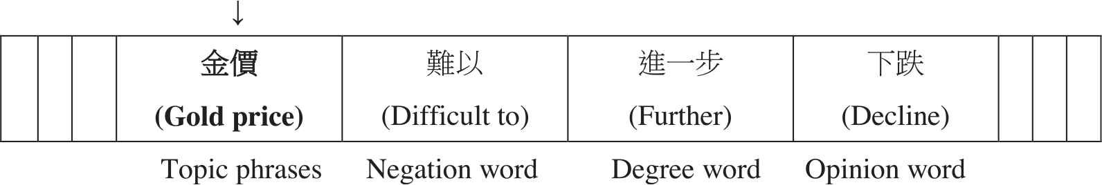
Topic phrase search in an example sentence.
Step 2. Taking the selected topic phrases as the center, go forward and backward to check 1–3 words to determine whether an opinion word is present in the opinion lexicon. If found, the two words “topic phrase” + “opinion polarity” are combined as a topic–opinion pair. Subsequently, go to Step 3, or go to check the next sentence. In Figure 3, an opinion word (下跌) is found; and the topic phrase polarity is “−.”
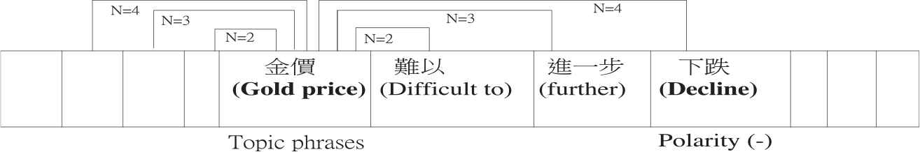
Opinion word search in an example sentence.
Step 3. Taking the selected opinion word as the center, go forward and backward to check 1–2 words to determine whether a negation word is present in the negation lexicon. If found, the opinion polarity is reversed; if not, go to Step 4. In Figure 4, a negation word (難以) is found; and the topic phrase polarity is reversed to “+.”
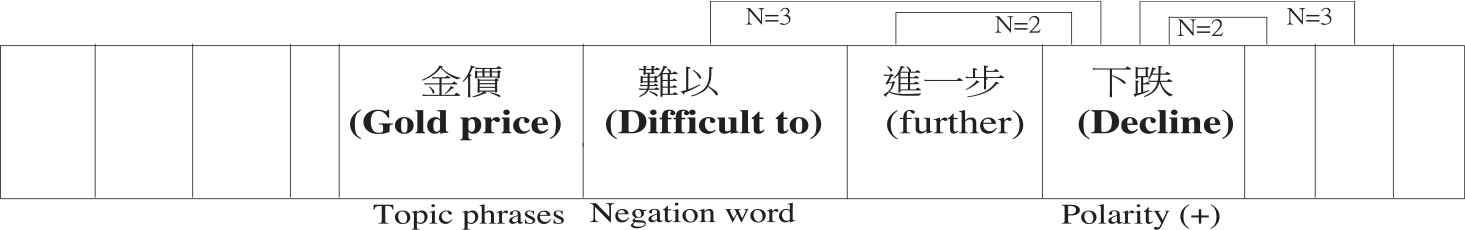
Negation word search in an example sentence.
Step 4. Taking the selected opinion word as the center, go forward and backward to check 1–2 words to determine whether a degree word is present in the HowNet lexicon. If found, sentiment strength is computed based on the degree (i.e., weight) predefined in HowNet. In Figure 5, a degree word (進一步) is found; and the defined weight in HowNet is used to compute the opinion score.
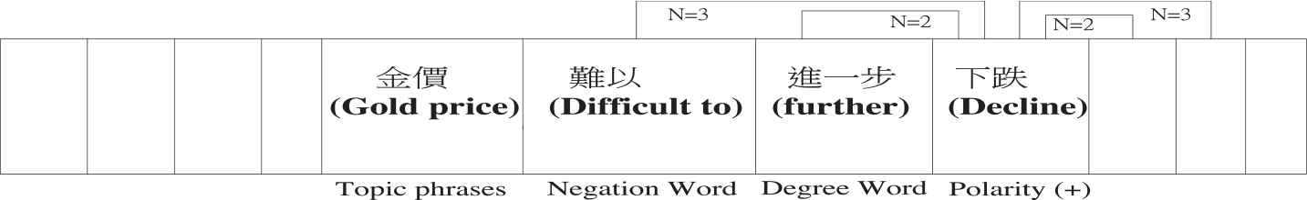
Degree word search in an example sentence.
Step 5. Continue Steps 1–4 until all sentences are checked.
2.5.3. Opinion score
To obtain an opinion value for topic phrases, Equation (9) is applied. The opinion score is computed on the basis of the polarity of the identified opinion words associated with topic phrases and the weight of degree words if they exist. The scoring function is defined as follows:
If a topic phrase A obtains a positive opinion score, it is interpreted as positively discussing the attribute. Similarly, if this sum is negative, it is interpreted as negatively discussing the attribute.
2.6. Variable Preprocessing
As already stated, the variables frequently used in the literature are collected and used in our prediction models, including gold spot prices; the prices of precious metals, such as silver, platinum, and palladium; the federal funds rate; the U.S. dollar index; crude oil prices; and the U.S. S&P 500 index. All variables and their sources are listed in Table 2.
| Economic Variable (Abbreviation) | Frequency | Sources | Explanation |
|---|---|---|---|
| GP | Daily | www.kitco.com | The price of gold is determined through trading in the gold and derivatives markets but a procedure known as The London Gold Fixing in the United Kingdom. |
| SP | Daily | www.kitco.com | A London silver price occurs daily where major international banks conduct and publish a fixing at noon London time. |
| PLP | Daily | www.quandl.com | The London Platinum and Palladium Market Fixing, sometimes referred to as the “London Fix,” is set each day at 09:45 (a.m. fix) and 14:00 (p.m. fix), London time. |
| PAP | Daily | www.quandl.com | Same as the platinum price. |
| Federal funds rate | Daily | www.investing.com | In the United States, the federal funds rate is the interest rate at which depository institutions lend reserve balances to other depository institutions overnight. |
| U.S. dollar Index | Daily | www.investing.com | The U.S. Dollar Index is an index of the value of the U.S. dollar relative to a basket of foreign currencies. |
| Crude oil Price | Daily | www.eia.gov | The crude oil price refers to the spot price of a barrel of benchmark crude oil. |
| U.S. S&P 500 Index | Daily | www.investing.com | This is a U.S. stock market index based on the market capitalizations of 500 large companies having common stock listed on the NYSE or NASDAQ. |
GP, gold price; PAP, palladium price; PLP, platinum price; SP, silver price, NYSE, New York Stock Exchange; NASDAQ, NASDAQ Composite Index.
Frequently used variables in gold prediction models.
2.7. Correlation Coefficient
A correlation coefficient is used in statistics to measure how strong a relationship is between two variables. There are several types of a correlation coefficient. The most common correlation coefficient is the Pearson Correlation Coefficient. It is known as the best method of measuring the association between variables of interest because it is based on the method of covariance. It gives information about the magnitude of the association, or correlation, as well as the direction of the relationship. The correlation coefficient formula is shown as Equation (10)
The ρ values range between −1.0 and 1.0. A correlation of −1.0 indicates a strong negative correlation, while a correlation of 1.0 indicates a strong positive correlation. A correlation of 0.0 indicates no relationship at all (https://www.statisticshowto.datasciencecentral.com/probability-and-statistics/correlation-analysis).
2.8. The Gold Price Forecasting Model Based on GA-LSSVR and Sentiment Analysis
The gold price forecasting model combining GA-LSSVR and sentiment analysis is constructed, as shown in Figure 6. First of all, the financial news is collected and preprocessed to do sentiment analysis and get an opinion score for each sentence. In the meantime, the frequently used variables, such as economic variables and precious metals, are collected and analyzed using correlation analysis to find the related predictors. The opinion scores and the selected predictors are combined and divided into training and testing data, then used in GA-LSSVR model to get the prediction result for each transaction set. Finally, the models are evaluated by using statistical analysis.
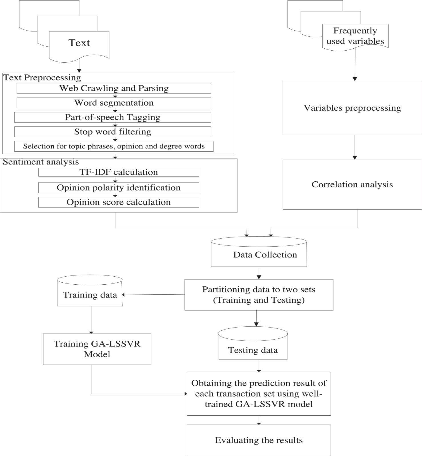
The flowchart of gold price forecasting model based on genetic algorithm-least square support vector regression (GA-LSSVR) and sentiment analysis.
3. EXPERIMENTAL RESULTS
3.1. Data
The daily gold spot price and frequently used economic variables listed in Table 2 are collected for the period 1/1/2016–12/31/2017 and undergo correlation analysis, as shown in Table 3. The variables with Pearson correlation coefficients >0.7 using Equation (10) are all precious metal prices, including gold price, silver price, platinum price, and palladium price, and are selected as input predictors. These selected predictors and opinion scores from opinion mining are used to test the model's performance, as presented in Table 4.
| Precious Metals and Economic Variables | Pearson Correlation Coefficient |
|---|---|
| Gold price | 0.984 |
| Silver price | 0.937 |
| Platinum price | 0.934 |
| Palladium price | 0.869 |
| Federal funds rate | −0.351 |
| U.S. dollar Index | −0.658 |
| Crude oil Price | 0.560 |
| U.S. S&P 500 Index | 0.108 |
Correlation analysis.
| Variable |
1 | 2 | 3 | 4 | 5 | Rolling Mechanism | Transaction Sets |
MAPE |
||||
|---|---|---|---|---|---|---|---|---|---|---|---|---|
| Model | 2016 | 2017 | 2016 |
2017 |
||||||||
| Mean | Std. | Mean | Std. | |||||||||
| 1 | GPt−1 | SP | PLP | PAP | Moved for 10 transaction dates | 24 | 25 | 0.014551 | 0.010834 | 0.017093 | 0.011600 | |
| 2 | GPt−1 | SP | PLP | PAP | OS | Moved for 10 transaction dates | 24 | 25 | 0.013627 | 0.010760 | 0.016472 | 0.011536 |
| 3 | GPt−1 | SP | PLP | PAP | Moved for 20 transaction dates | 11 | 12 | 0.018539 | 0.014579 | 0.017864 | 0.010117 | |
| 4 | GPt−1 | SP | PLP | PAP | OS | Moved for 20 transaction dates | 11 | 12 | 0.018386 | 0.014320 | 0.025658 | 0.015455 |
MAPE, mean absolute percentage error; PAP, palladium price; PLP, platinum price; SP, silver price; OS, Opinion Score.
GPt−1: previous gold price.
Prediction results of each forecasting model.
In our forecasting model, data sets are divided into training and test sets and moved using a rolling mechanism: (1) moved for ten transaction dates; (2) moved for 20 transaction dates. The structure of the rolling mechanism is illustrated in Figure 7. The transaction dates are counted and marked as transaction numbers. In 2016 and 2017, 250 and 260 transaction numbers are present, respectively. On the basis of the first rolling mechanism, 24 and 25 transaction sets are present in 2016 and 2017, respectively. Based on the second rolling mechanism, 11 and 12 transaction sets are present in 2016 and 2017, respectively. To evaluate the forecasting performance, the training data set is used to identify the optimal forecasting model, and the testing data set is used to appraise the forecasting model's performance.
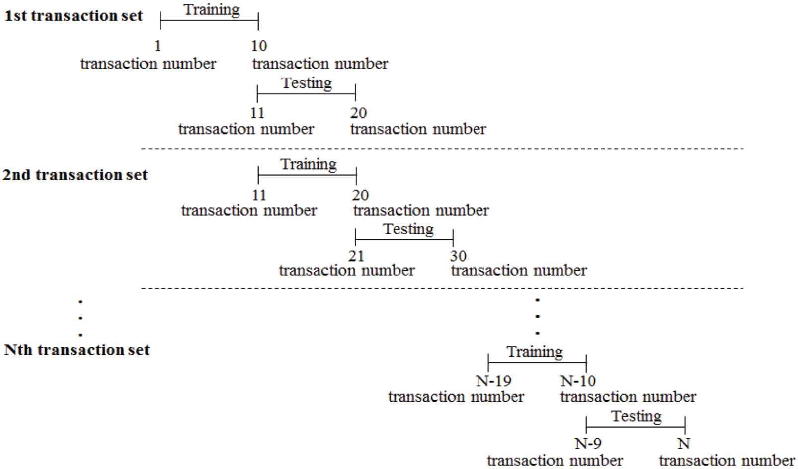
Rolling mechanism based on being “moved for ten transaction dates” (nontrading days excluded).
3.2. Opinion Mining
In total, 5450 news (433052 sentences) pieces are identified, including date, title, and content automatically crawled from cnYES in Taiwan, from January 1, 2016, to December 31, 2017. Table 5 describes the data set.
| Year | Documents | Sentences | Labeled Sentences | Positive | Negative |
|---|---|---|---|---|---|
| 2016 | 1270 | 65213 | 4590 | 1933 | 2657 |
| 2017 | 4180 | 367839 | 11829 | 5990 | 5839 |
| Total | 5450 | 433052 | 16419 | 7923 | 8496 |
Data set descriptions.
3.2.1. Selected topic phrases based on TF–IDF
To evaluate topic phrases, TF–IDF is used. Table 6 presents the results. The results indicate that “黃金 (gold)” and “金價 (gold price)” have the optimal TF–IDF. Therefore, “黃金 (gold)” and “金價 (gold prices)” are selected as topic phrases.
| Topic Phrases | TF-IDF |
|---|---|
| 黃金 (Gold) | 0.0091 |
| 金價 (Gold price) | 0.0042 |
TF-IDF, Term Frequency–Inverse Document Frequency.
Topic phrases.
3.2.2. Selected positive phrases based on TF–IDF
Forty-four positive phrases with TF–IDF exceeding 0.000005 are selected, and the top 10 are listed in Table 7 as examples.
| Positive Phrases | TF-IDF |
|---|---|
| 高點 (high) | 0.001535 |
| 強勢 (strong) | 0.001333 |
| 漲幅 (increase) | 0.001099 |
| 上漲 (grow) (progress) (extend) (expand) (rise) | 0.005231 |
| 上升 (rise) | 0.002021 |
| 強勁 (on fire) | 0.000889 |
| 回升 (rally) | 0.000844 |
| 拉升 (ramping) | 0.000796 |
| 走高 (go up) | 0.000790 |
| 看漲 (bullish) | 0.000762 |
TF-IDF, Term Frequency–Inverse Document Frequency.
Top 10 positive phrases.
3.2.3. Selected negative phrases based on TF–IDF
Forty-eight negative phrases with TF–IDF exceeding 0.000005 are selected, and the top 10 are listed in Table 8 as examples.
| Negative Phrases | TF-IDF |
|---|---|
| 跌掉 (fell) | 0.000009 |
| 慘跌 (plummet) | 0.000022 |
| 看淡 (bearish) | 0.000036 |
| 跌停 (touch the downward price limit) | 0.000043 |
| 重壓 (pressure) | 0.000047 |
| 崩跌 (collapse) (slump) (go bust) | 0.000052 |
| 重挫 (plunge) | 0.000374 |
| 滑落 (slip) | 0.000058 |
| 下挫 (fell) | 0.000973 |
| 拖累 (encumber) | 0.000423 |
TF-IDF, Term Frequency–Inverse Document Frequency.
Top 10 negative phrases.
3.2.4. Opinion score
The daily opinion scores of gold news from January 2016 to December 2017 are calculated on the basis of Equation (9) and the amount by month is added, as shown in Table 9, and normalized with the average monthly actual gold price using Equation (11), as illustrated in Figure 8. Figure 8 reveals that the monthly opinion score and average monthly actual gold price trends are the same.
| Transaction Year | Transaction Month | Monthly Opinion Score | Average Monthly Actual Gold Price |
|---|---|---|---|
| 2016 | Jan | 107 | 1262.85 |
| Feb | −42 | 1189.76 | |
| Mar | −45 | 1191.00 | |
| Apr | −37 | 1197.43 | |
| May | −34 | 1188.75 | |
| Jun | −69 | 1170.58 | |
| Jul | −320 | 1102.41 | |
| Aug | −90 | 1125.89 | |
| Sep | −78 | 1141.54 | |
| Oct | 30 | 1132.51 | |
| Nov | −72 | 1070.20 | |
| Dec | −139 | 1080.88 | |
| 2017 | Jan | 70 | 1145.00 |
| Feb | 287 | 1239.62 | |
| Mar | 89 | 1235.13 | |
| Apr | 36 | 1265.31 | |
| May | −123 | 1246.74 | |
| Jun | 179 | 1322.11 | |
| Jul | 217 | 1339.04 | |
| Aug | 165 | 1329.41 | |
| Sep | 88 | 1294.90 | |
| Oct | −108 | 1269.95 | |
| Nov | −87 | 1181.38 | |
| Dec | −249 | 1154.03 |
Opinion scores of gold news from January 2016 to December 2017.

Comparison of monthly opinion scores and gold prices for 2016–2017.
3.3. Simulation Results
The solutions for the gold price forecasting are obtained using the GA-LSSVR algorithm as described in the previous section. The GA portion is implemented in MATLAB, and the LSSVR portion is performed using LIBSVM (the LSSVM tool box) [56]. The parameter settings for GA are listed in Table 10.
| Parameter | Value |
|---|---|
| Population size | 100 |
| Number of parameters | 2 |
| Selection method | Tournament |
| Mutation ratio | 0.05 |
| Generations | 1000 |
| Elitism | 2 chromosomes |
GA, genetic algorithm.
Required GA parameters.
As explained, in a particular run for the second transaction set of model 2 in 2016 (Table 11), the GA-LSSVR steps continue up to the maximum of 1000 generations with the MAPE convergence, as visualized in Figure 9. The run of the test MAPE used the parameter value C = 979.93 and Kernel variable = 839.53. Table 12 presents the real gold price and test prediction results from the LSSVR regression. The real gold prices and test prediction values are provided in Figure 10.
| Year |
2016 |
2017 |
||||||||
|---|---|---|---|---|---|---|---|---|---|---|
| Model |
Moved for 10 Transaction Dates |
Moved for 20 Transaction Dates |
Moved for 10 Transaction Dates |
Moved for 20 Transaction Dates |
||||||
| Transaction Set | Model 1 | Model 2 | Model 3 | Model 4 | Model 1 | Model 2 | Model 3 | Model 4 | ||
| 1 | 0.017553 | 0.013337 | 0.040662 | 0.042266 | 0.058380 | 0.057069 | 0.012982 | 0.013370 | ||
| 2 | 0.016119 | 0.014309 | 0.009550 | 0.008269 | 0.011811 | 0.010226 | 0.008646 | 0.009822 | ||
| 3 | 0.024240 | 0.024047 | 0.009967 | 0.010004 | 0.021160 | 0.013047 | 0.023707 | 0.023230 | ||
| 4 | 0.008032 | 0.011684 | 0.011234 | 0.010917 | 0.012721 | 0.012961 | 0.018465 | 0.023995 | ||
| 5 | 0.014060 | 0.010110 | 0.006455 | 0.007265 | 0.007239 | 0.005103 | 0.019990 | 0.053462 | ||
| 6 | 0.005901 | 0.005317 | 0.010918 | 0.011435 | 0.009553 | 0.009730 | 0.006400 | 0.008622 | ||
| 7 | 0.008070 | 0.008069 | 0.010787 | 0.010006 | 0.021055 | 0.021061 | 0.006223 | 0.008880 | ||
| 8 | 0.014696 | 0.014696 | 0.017301 | 0.018450 | 0.007574 | 0.007462 | 0.014328 | 0.017465 | ||
| 9 | 0.013387 | 0.013181 | 0.025677 | 0.025256 | 0.021817 | 0.024973 | 0.020261 | 0.032302 | ||
| 10 | 0.006191 | 0.006306 | 0.050894 | 0.048284 | 0.034664 | 0.035857 | 0.040596 | 0.048189 | ||
| 11 | 0.008220 | 0.008419 | 0.010479 | 0.010096 | 0.007352 | 0.007150 | 0.012684 | 0.041510 | ||
| 12 | 0.028870 | 0.025448 | 0.026167 | 0.018814 | 0.030087 | 0.027054 | ||||
| 13 | 0.011006 | 0.010997 | 0.006589 | 0.006241 | ||||||
| 14 | 0.021915 | 0.012907 | 0.009967 | 0.010453 | ||||||
| 15 | 0.017308 | 0.007702 | 0.010515 | 0.010517 | ||||||
| 16 | 0.010316 | 0.013048 | 0.010515 | 0.010254 | ||||||
| 17 | 0.008672 | 0.008296 | 0.007107 | 0.007109 | ||||||
| 18 | 0.018231 | 0.016257 | 0.020384 | 0.020387 | ||||||
| 19 | 0.007467 | 0.008244 | 0.016689 | 0.017005 | ||||||
| 20 | 0.055908 | 0.057218 | 0.008646 | 0.009249 | ||||||
| 21 | 0.005123 | 0.004983 | 0.029436 | 0.029435 | ||||||
| 22 | 0.006770 | 0.006774 | 0.015716 | 0.015081 | ||||||
| 23 | 0.006309 | 0.006309 | 0.009018 | 0.008650 | ||||||
| 24 | 0.014851 | 0.019391 | 0.020521 | 0.020744 | ||||||
| 25 | 0.022738 | 0.023233 | ||||||||
MAPE, mean absolute percentage error.
The MAPEs for each model.
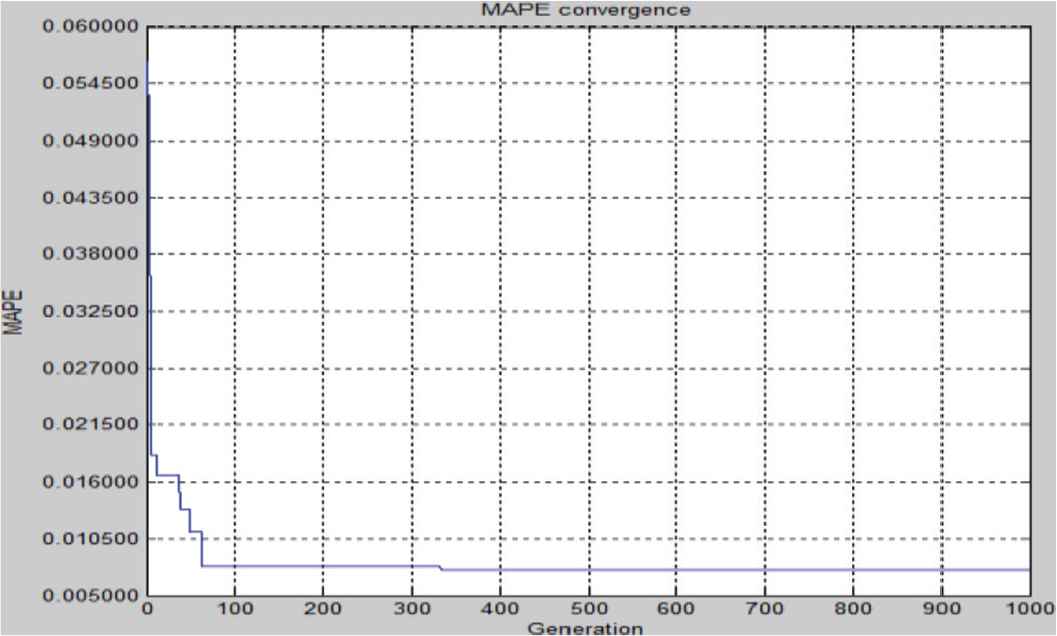
Mean absolute percentage error (MAPE) convergence for the second transaction set of model 2 in 2016.
| Transaction Number | Actual Gold Price | Forecasted Gold Price |
|---|---|---|
| 21 | 1209.50 | 1240.02 |
| 22 | 1206.00 | 1234.70 |
| 23 | 1209.50 | 1228.85 |
| 24 | 1208.25 | 1228.77 |
| 25 | 1204.50 | 1233.28 |
| 26 | 1192.50 | 1224.06 |
| 27 | 1204.75 | 1218.51 |
| 28 | 1208.25 | 1224.19 |
| 29 | 1214.00 | 1209.19 |
| 30 | 1212.50 | 1217.31 |
| MAPE | 0.014309 |
LSSVR, least square support vector regression; MAPE, mean absolute percentage error.
Actual gold price and LSSVR predictions.
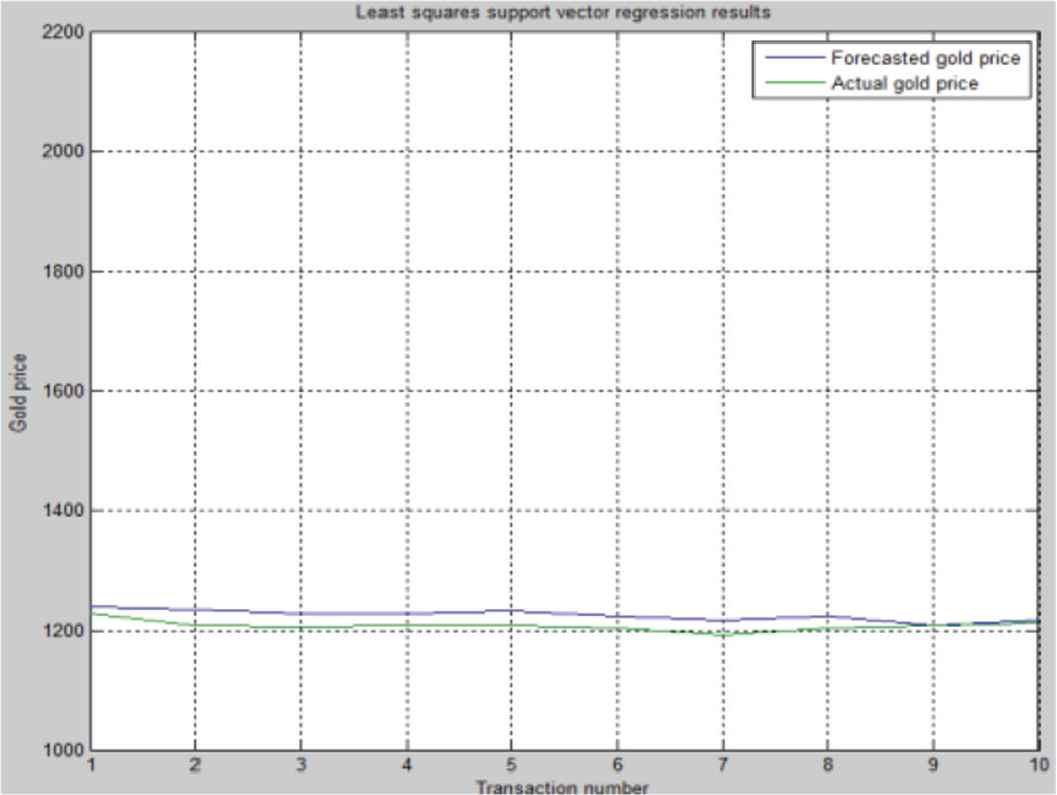
Genetic algorithm-least square support vector regression (GA-LSSVR) results for the second transaction set of model 2 in 2016.
After the intensive experimental test for each transaction set, the prediction results of the forecasting models based on previous gold prices and various combinations of variables for the period 2016–2017 are summarized in Table 11. The prediction results of each forecasting model for the various variables and the rolling mechanism is presented in Table 4.
Table 11 reports the MAPE results for each forecasting model based on the rolling mechanism. The mean values (mean) and standard deviation (Std.) of MAPE are given in Table 4. On the basis of the experiments, this study concludes that the most accurate model stressed in boldface with the smallest Mean and Std. of MAPE is the one that uses previous gold price, the precious metals, including silver price (SP), platinum price (PLP), and palladium price (PAP), and opinion scores' variables on the basis of the rolling mechanism moves for 10 transaction dates. First, the standard deviations (Std.) of Model 2s' MAPEs are quite small. This indicates that the predetermined variables have a slight impact on the prediction of the GA-LSSVR model. Second, the Model 2 can obtain the smallest mean values (mean) of MAPEs, which repeatedly confirms the effectiveness of Model 2. Finally, this experiment proves that the opinion scores can improve the accuracy of gold price forecasting for shorter trading days (i.e., moved for ten transaction dates) in terms of MAPE.
Furthermore, two statistical tests, Wilcoxon test [11,57] and Friedman test [10,11,58], are also conducted to ensure the significant contribution in terms of forecasting accuracy improvement for the Model 2. The two test results are illustrated in Table 13 that the Model 2 almost reaches significance level in terms of forecasting performance than other alternative compared models.
| Wilcoxon Test (α = 0.05) |
Friedman Test | |||
|---|---|---|---|---|
| Model 2 vs. | R+ | R− | p Value | (α = 0.05) |
| Model 1 | 0 | 3 | 0.0074 | H0: e1 = e2 = e3 = e4 |
| Model 3 | 0 | 3 | 0.0074 | F = 111.6 |
| Model 4 | 0 | 3 | 0.0074 | P = 0.0000 (reject H0) |
Results of Wilcoxon test and Friedman test for Model 2 against compared models.
The Friedman test is a multiple comparisons test that aims to detect significant differences between the results of two or more algorithms/models. The statistic F of the Friedman test is shown as Equation (12),
In this study, the Wilcoxon test is employed using Equation (13). Table 13 also summarizes the results of applying Wilcoxon test. It displays the sum of rankings obtained in each comparison and the p-value associated.
As stated in García et al., [57] when performing multiple pair-wise tests, to avoid losing the control on the Family Wise Error Rate (FWER), the true statistical significance for combining pair-wise comparisons must be given by:
From expression (14) and Table 13, we can deduce that Model 2 is better than the other compared models with a p-value of
Hence, once again the statistical analysis proves Model 2 really outperforms the three compared models considering independent pair-wise comparisons due to the fact that the p-value is below α = 0.05.
4. THE DISCUSSION AND CONCLUSION
Gold is used as an investment and hedging tool. The investment industry is changing rapidly, especially in gold investment. To reduce investment risk, investors must establish an effective gold price forecasting system. In this study, the opinion scores obtained from text mining are combined with the precious metals' prices selected from conventional variables as predictors to predict gold prices using GA-LSSVR model. The study results showed that the prediction performance is enhanced.
Most studies that investigate the causes of variations in gold prices determine that the main drivers are hard economic factors. Those economic indicators are lagging indicators. However, some studies suggest that using lagging indicators in forecasting models is ineffective. This study is the first to use the opinion score as an input predictor to forecast short-term gold prices. The gold price depends largely on confidence in the current market. Opinion scores represent the current market trends. They have become effective forecasting indicators. Our experimental results indicate that using opinion score as an input predictor to forecasting models can result in more accurate prediction results than those without it for short-term gold price forecasting. The use of opinion score allowed the identification of nonquantitative factors that affected the forecasting model and must be investigated in the forecasting model to improve the predicting ability.
Furthermore, in this study, a GA-LSSVR is applied to forecast gold prices using opinion scores and the selected precious metals' prices as predictors. In the GA-LSSVR model, the GA is used to select the optimal parameters of LSSVR, and the MAPE method is used to evaluate the fitness. In this research, the gold prices from daily transactions, commonly used conventional variables, and opinion scores from 2016 to 2017 were collected and used as our research data. By using the selected precious metals' prices and opinion scores with the rolling mechanism moving for 10 transaction dates, the experimental results have shown that GA-LSSVR achieves superior forecasting accuracy. In the future, we would like to apply the sentiment analysis to the forecasting models to improve the forecasting performance for decision-makers' references.
CONFLICT OF INTEREST
There is no “Conflict of Interest” issue.
ACKNOWLEDGMENTS
The author thanks the National Science Council of Taiwan, R.O.C., for financially supporting this research under contract MOST104-2410-H-155-038.
REFERENCES
Cite this article
TY  - JOUR
AU  - Fong-Ching Yuan
AU  - Chao-Hui Lee
AU  - Chaochang Chiu
PY  - 2020
DA  - 2020/02/23
TI  - Using Market Sentiment Analysis and Genetic Algorithm-Based Least Squares Support Vector Regression to Predict Gold Prices
JO  - International Journal of Computational Intelligence Systems
SP  - 234
EP  - 246
VL  - 13
IS  - 1
SN  - 1875-6883
UR  - https://doi.org/10.2991/ijcis.d.200214.002
DO  - 10.2991/ijcis.d.200214.002
ID  - Yuan2020
ER  -