International Journal of Computational Intelligence Systems

Volume 13, Issue 1, 2020, Pages 1 - 11

Almost Automorphic Solutions to Cellular Neural Networks With Neutral Type Delays and Leakage Delays on Time Scales

Authors
Changjin Xu1, *, Maoxin Liao2, Peiluan Li3, Zixin Liu4
1Guizhou Key Laboratory of Economics System Simulation, Guizhou University of Finance and Economics, Guiyang 550004, PR China
2School of Mathematics and Physics, University of South China, Hengyang 421001, PR China
3School of Mathematics and Statistics, Henan University of Science and Technology, Luoyang 471023, PR China
4School of Mathematics and Statistics, Guizhou University of Finance and Economics, Guiyang 550004, PR China
*Corresponding author. Email: xcj403@126.com
Corresponding Author
Changjin Xu
Received 4 August 2019, Accepted 2 January 2020, Available Online 15 January 2020.
DOI
10.2991/ijcis.d.200107.001How to use a DOI?
Keywords
Cellular neural networks; Almost automorphic solution; Exponential stability; Leakage delay; Neutral type delay
Abstract

In this paper, cellular neural networks (CNNs) with neutral type delays and time-varying leakage delays are investigated. By applying the existence of the exponential dichotomy of linear dynamic equations on time scales, a fixed point theorem and the theory of calculus on time scales, a set of sufficient conditions which ensure the existence and exponential stability of almost automorphic solutions of the model are obtained. An example with its numerical simulations is given to support the theoretical findings.

Copyright
© 2020 The Authors. Published by Atlantis Press SARL.
Open Access
This is an open access article distributed under the CC BY-NC 4.0 license (http://creativecommons.org/licenses/by-nc/4.0/).

1. INTRODUCTION

Since the cellular neural networks with delay were first introduced and investigated by Roska and Chua [1], they have been extensively applied in various different fields such as classification of pattern and processing of moving images. In recent years, extensive results on the existence and stability of equilibrium points, periodic solutions, almost periodic solutions and anti-periodic solutions for cellular neural networks have been reported. For example, Fan and Shao [2] investigated the positive almost periodic solutions for shunting inhibitory cellular neural networks with time-varying and continuously distributed delays, Li and Wang [3] analyzed the existence and exponential stability of the almost periodic solutions of shunting inhibitory cellular neural networks on time scales, Xia et al. [4] established the sufficient conditions for the existence and exponential stability of almost periodic solution for shunting inhibitory cellular neural networks with impulses, Peng and Wang [5] addressed the existence and exponential stability of anti-periodic solutions to shunting inhibitory cellular neural networks with time-varying delays in leakage terms. For more related work on shunting inhibitory cellular neural networks, one can see [4, 617].

Many scholars [1821] argue that neural networks usually contain some information about the derivative of the past state to further describe and model the dynamics for the complex neural reactions. Then some authors focused on the dynamical behaviors of neutral type neural networks. For example, Rakkiyappan et al. [22] considered the global exponential stability for neutral-type impulsive neural networks, Li et al. [23] discussed the existence of periodic solutions for neutral type cellular neural networks with delays, Bai [24] investigated the global stability of almost periodic solutions of Hopfield neural networks with neutral time-varying delays. In details, we refer the reader to [2530].

Very recently, a typical time delay called Leakage (or “forgetting”) delay may exist in the negative feedback terms of the neural network system, and these terms are variously known as forgetting or leakage terms [31,32]. Since time delays in the leakage term are difficult to handle but have great impact on the dynamical behavior of neural networks. Therefore, it is meaningful to consider neural networks with time delays in leakage terms [34].

It is well known that both continuous time and discrete time neural networks play an equal roles in various applications [34]. But it is troublesome to study the dynamical properties for continuous and discrete time systems, respectively. In 1990, Hilger [35] proposed the theory of time scales which can deal with both difference and differential calculus in a consistent way. Thus it is significant to investigate the dynamical behaviors of neural networks on time scales. For instance, some authors [3,3640] investigated periodic solutions, almost periodic solutions and anti-periodic solutions of some neural networks on time scales.

In addition, we shall point out that in real word, almost periodicity is universal than periodicity. Moreover, almost automorphic functions, which were introduced by Bochner, are much more general than almost periodic functions. In addition, the almost automorphic solutions of neural networks can be applied in many areas such as automatic control, image processing, psychophysics, robotics and so on [4145]. Almost automorphic solutions in the context of differential equations were studied by several authors. We refer the reader to [4653]. However, to the best of our knowledge, there is no paper published on the almost automorphic solutions of cellular neural networks with neutral type delays and time-varying leakage delays on time scales.

Inspired by the discussion above, in this paper, we consider the following cellular neural networks with neutral type delays and time-varying leakage delays on time scales

xiΔ(t)=bi(t)xi(tηi(t))+j=1naij(t)fj(xj(t))+j=1nbij(t)fj(xj(tτij(t)))+j=1ncij(t)fj(xiΔ(tσij(t)))+Ii(t),(1)
where T is an almost periodic time scale, i=1,2,,n, n corresponds to the number of units in a neural network, xi corresponds to the state vector of the ith unit at time t, fj(xj(t)) denotes the output of the jth unit on ith unit at time t, bij denotes the strength of the jth unit on the ith unit at time tτij, Ii denotes the external bias on the ith unit at time t, τij corresponds to the transmission delay along the axon of the jth unit, bi represents the rate with which the ith unit will reset its potential to the resting state in isolation when disconnected from the network and external inputs, ηi>0 with tηi(t)T for all tT denote s time delay in leakage term, τij(t)0,σij(t)0 correspond the transmission delays and satisfy that for tT,tτijT,tσijT.

The main aim of this article is to establish some sufficient conditions for the existence and global exponential stability of almost automorphic periodic solutions of (1). By applying the existence of the exponential dichotomy of linear dynamic equations on time scales, a fixed point theorem and the theory of calculus on time scales, we obtain a set of sufficient conditions for the existence and exponential stability of almost automorphic solutions for model (1).

For convenience, we denote by [a,b]T={t|t[a,b]T}. For a almost automorphic function f:TR, f+=suptR|f(t)|,f=inftR|f(t)|. We denote by R the set of real numbers, by R+ the set of positive real numbers, by X a real Banach space with the norm ||.||. The initial conditions associated with system (1) are of the form:

xi(s)=φi(s),xiΔ(s)=φiΔ(s),s(τ,0]T,(2)
where τ=max{max1inηi+,max(i,j){τij+,σij+}},φiC1([τ,0]T,R) and i,j=1,2,,n.

The remainder of the paper is organized as follows. In Section 2, we introduce some lemmas and definitions, which can be used to check the existence of almost automorphic solutions of system (1). In Section 3, we present some sufficient conditions for the existence of almost automorphic solutions of (1). Some sufficient conditions on the global exponential stability of almost automorphic solutions of (1) are established in Section 4. An example is given to illustrate the effectiveness of the obtained results in Section 5. A brief conclusion is drawn in Section 6.

2. PRELIMINARY RESULTS

In this section, we would like to recall some basic definitions and lemmas which are used in what follows.

Definition 2.1.

[54] Let T be a nonempty closed subset (time scale) of R. The forward and backward jump operators σ,ρ:TT and the graininess μ:TR are defined, respectively, by

σ(t)=inf{sT:s>t},ρ(t)=sup{sT:s<t} and μ(t)=σ(t)t.

Lemma 2.1.

[54] Assume that p,q:TR are two regressive functions, then

  1. e0(t,s)1 and ep(t,t)1;

  2. ep(t,s)=1ep(s,t)=ep(s,t);

  3. ep(t,s)ep(s,r)=ep(t,r);

  4. (ep(t,s))Δ=p(t)ep(t,s).

Lemma 2.2.

[54] Let f,g be Δ-differentiable functions on T, then

  1. (ν1f+ν2g)Δ=ν1fΔ+ν2gΔ, for any constants ν1,ν2;

  2. (fg)Δ(t)=fΔ(t)g(t)+f(σ(t))gΔ(t)=f(t)gΔ(t)+fΔ(t)g(σ(t)).

Lemma 2.3.

[54] Assume that p(t)0 for ts, then ep(t,s)1.

Definition 2.2.

[54] A function p:TR is called regressive provided 1+μ(t)p(t)0 for all tTk; p:TR is called positively regressive provided 1+μ(t)p(t)>0 for all tTk. The set of all regressive and rd-continuous functions p:TR will be denoted by R=R(T,R) and the set of all positively regressive functions and rd-continuous functions will be denoted by R+=R+(T,R).

Lemma 2.4.

[54] Suppose that pR+, then

  1. ep(t,s)>0, for all t,sT;

  2. if p(t)q(t) for all ts, then ep(t,s)eq(t,s) for all ts.

Lemma 2.5.

[54] If pR and a,b,cT, then

[ep(c,.)]Δ=p[ep(c,.)]σ
and
abp(t)ep(c,σ(t))Δt=ep(c,a)ep(c,b).

Lemma 2.6.

[54] Let aTk,bT and assume that f:T×TkR is continuous at (t,t) where tTk with t>a. Also assume that fΔ(t) is rd-continuous on [a,σ(t)]. Suppose that for each ε>0, there exists a neighborhood U of ϵ[a,σ(t)] such that

|f(σ(t),ϵ)f(s,ϵ)fΔ(t,ϵ)(σ(t)s)|ε|σ(t)s|,for allsU,
where fΔ denotes the derivative of f with respect to the first variable. Then
  1. g(t):=atf(t,ϵ)Δϵ implies gΔ(t):=atfΔ(t,ϵ)Δϵ+f(σ(t),t);

  2. h(t):=tbf(t,ϵ)Δϵ implies hΔ(t):=tbfΔ(t,ϵ)Δϵf(σ(t),t).

Next, we recall some definitions of almost automorphic functions on time scales.

Definition 2.3.

[55] A time scale T is called an almost periodic time scale if

Π:={ϵR:t±ϵT,tT{0}.

Definition 2.4.

[54] Let T be an almost periodic time scale.

  1. A function f(t):TX is said to be almost automorphic, if for any sequence {sn}n=1Π, there is a subsequence{ϵn}n=1{sn}n=1 such that g(t)=limnf(t+ϵn) is well defined for each tT and limng(tϵn)=f(t) for each tT. Denote by AA(T,X) the set of all such functions;

  2. A continuous function f:T×XX is said to be almost automorphic, if f(t,x) is almost automorphic in tT uniformly in xB, where B is any bounded subset of X. Denote by AA(T×X,X) the set of all such functions.

Lemma 2.7.

[53] Let f,gAA(T,X). Then we have the following

  1. f+gAA(T,X);

  2. αAA(T,X) for any constant αR;

  3. if φ:XY is a continuous function, then the composite function φf:TY is almost automorphic.

Lemma 2.8.

[34] Let fAA(T×X,X) and f satisfies the Lipschitz condition in xX uniformly in tT. If φAA(T,X), then f(t,φ(t)) is almost automorphic.

Definition 2.5.

[55] Let xRn and A(t) be a n×n matrix-valued function on T, the linear system

xΔ(t)=A(t)x(t),tT(3)
is said to admit an exponential dichotomy on T if there exist positive constants ki,αi,i=1,2, projection P and the fundamental solution matrix X(t) of (3) satisfying
|X(t)PX1(s)|k1eα1(t,s),s,tT,ts
and
|X(t)(IP)X1(s)|k2eα2(t,s),s,tT,ts,
where |.| is a matrix norm on T, that is, if A=(aij)n×n, then we can take |A|=(i=1nj=1n|aij|2)12.

Lemma 2.9.

[53] Suppose that A(t)AA(T,Rn×n) such that {A1(t)}tT and {((I+μ(t))A(t))1}tT are bounded. Moreover, suppose that gAA(T,Rn) and (3) admits an exponential dichotomy, then the following system

xΔ(t)=A(t)x(t)+g(t)(4)
has a solution x(t)AA(T,Rn) and x(t) is expressed as follows
x(t)=tX(t)PX1(σ(s))g(s)Δst+X(t)(IP)X1(σ(s))g(s)Δs,
where X(t) is the fundamental solution matrix of (3), I denotes the n×n-identity matrix.

Lemma 2.10.

[55] Let ci>0 and ci(t)R+,tT. If min1in{inftTci(t)}=m>0, then the linear system

xΔ(t)=diag(c1(t),c2(t),,cn(t))x(t)(5)
admits an exponential dichotomy on T.

Definition 2.6.

[34] Let x(t)=(x1(t),x2(t),,xn(t))T be an almost automorphic solution of (1) with initial value φ(t)=(φ1(t),φ2(t), ,φn(t))T. If there exist positive constants λ with λR+ and M>1 such that for an arbitrary solution x(t)=(x1(t),x2(t),,xn(t))T of (1) with initial value φ(t)=(φ1(t),φ2(t),,φn(t))T satisfies

||xx||M||φφ||eλ(t,t0),t0[τ,)T,tt0.

Then the solution x(t) is said to be globally exponentially stable.

3. EXISTENCE OF ALMOST AUTOMORPHIC SOLUTIONS

In this section, we will establish sufficient conditions on the existence of pseudo almost periodic solutions of (1). Let X={fC1(T,R|f,fΔAA(T,Rn)} with the norm ||f||X=max{|f|1,|fΔ|1}, where |f|1=max1infi+,|fΔ|1=max1in(fiΔ)+. Then X is a Banach space. Let φ0(t)=(φ10(t),φ20(t),,φn0(t))T , where φi0(t)=tebi(t,σ(s)Ii(s)Δs),i=1,2,,n and L be a constant satisfying Lmax{||φ0||X,max1in{fj(0)}}. Throughout this article, we assume that

(H1) biC(T,R+) with biR+ and inftT{1μ(t)bi(t)}=b̄>0,aij,bij,cij,IiC(T,R), τij,σijC(T,R+) are almost automorphic, where i,j=1,2,,n.

(H2) fjC(R,R) and there exist constants Lj>0 and Mj>0 such that for any u,vR,

|fj(u)fj(v)|Lj|uv|,|fj(u)|Mj,
where j=1,2,,n.

(H3)

max1inϱibi,1+bi+biϱi12,max1inςibi,1+bi+biςi1
where
ϱi=bi+ηi++j=1n(aij++bij++cij+)(Lj+1),ςi=bi+ηi++j=1n[(aij++bij++cij+)Lj].

Theorem 3.1.

If (H1)–(H3) are satisfied. Then there exists a unique almost automorphic solution of system (1) in X0={φX|||φφ0||XL}.

Proof

For any given φX, we consider the following system

xiΔ(t)=bi(t)xi(t)+Θi(t,φ)+Ii(t),i=1,2,,n,(6)
where
Θi(t,φ)=bi(t)tηi(t)tφiΔ(s)Δs+j=1naij(t)fj(φj(t))+j=1nbij(t)fj(φj(tτij(t)))+j=1ncij(t)fj(φiΔ(tσij(t))),i=1,2,,n.(7)

It follows from Lemma 2.10 that the linear system

xiΔ(t)=bi(t)xi(t),i=1,2,,n,(8)
admits an exponential dichotomy on T. Thus, in view of Lemma 2.9, we derive that system (6) has exactly one almost automorphic solution as follows
xiφ(t)=tebi(t,σ(s))[Θi(s,φ)+Ii(s)]Δs,i=1,2,,n,(9)

For φX, then

||φ||X||φφ0||X+||φ0||X2L.(10)

Define an operator as follows

Φ:XX,(φ1,φ2,,φn)T(x1φ,x2φ,,xnφ)T.(11)

First we show that for any φX, we have ΦφX. Note that, for i=1,2,,n, we have

|Θi(s,φ)=|bi(s)sηi(s)sφiΔ(θ)Δθ+j=1naij(s)fj(φj(s))+j=1nbij(s)fj(φj(sτij(s)))+j=1ncij(s)fj(φiΔ(sσij(s)))|
bi+ηi+||φ||X+j=1naij+(|fj(φj(s))fj(0)|+|fj(0)|)+j=1nbij+(|fj(φj(sτij(s)))fj(0)|+|fj(0)|)+j=1ncij+(|fj(φiΔ(sσij(s)))fj(0)|+|fj(0)|)bi+ηi+||φ||X+j=1naij+(Lj||φ||X+|fj(0)|)+j=1nbij+(Lj||φ||X+|fj(0)|)+j=1ncij+(Lj||φ||X+|fj(0)|)=[bi+ηi++j=1n(aij++bij++cij+)Lj]||φ||X+j=1n[aij++bij++cij+)|fj(0)|]2L{bi+ηi++j=1n[(aij++bij++cij+)(Lj+1)]}.(12)

Thus we get

|(Φ(φφ0))i(t)|=|tebi(t,σ(s))Θi(s,φ)Δs|tebi(t,σ(s))|Θi(s,φ)|Δs2Ltebi(t,σ(s))bi+ηi++j=1n[(aij++bij++cij+)(Lj+1)]Δs2Lϱibi,i=1,2,,n.(13)

On the other hand, for i=1,2,,n, we have

|(Φ(φφ0))iΔ(t)|=|(tebi(t,σ(s))Θi(s,φ)Δs)tΔ|=|Θi(t,φ)bi(t)tebi(t,σ(s))Θi(s,φ)Δs||Θi(t,φ)|+|bi(t)|tebi(t,σ(s))|Θi(s,φ)|Δs2Lϱi(1+bi+bi),i=1,2,,n.(14)

It follows from (H3) that

||Φφφ0||Xmax1inϱibi,1+bi+biϱiL(15)
which implies that ΦφX. Next, we show that Φ is a contraction. For any φ=(φ1,φ2,,φn)T,ψ=(ψ1,ψ2,,ψn)TX, for i=1,2,,n, we denote
ϒi(s,φ,ψ)=bi(t)sηi(s)s(φiΔ(s)ψiΔ(s))Δs+j=1naij(t)[fj(φj(t))fj(ψj(t))]+j=1nbij(t)[fj(φj(tτij(t)))fj(ψj(tτij(t)))]+j=1ncij(t)[fj(φiΔ(tσij(t)))fj(ψiΔ(tσij(t)))].(16)

Then

|(ΦφΦψ)i(t)|=|tebi(t,σ(s))ϒi(s,φ,ψ)Δs|tebi(t,σ(s))|ϒi(s,φ,ψ)|Δstebi(t,σ(s)){bi+ηi++j=1n[(aij++bij++cij+)Lj]}Δs||φψ||Xςibi||φψ||X,i=1,2,,n(17)
and
|(ΦφΦψ)iΔ(t)|=|tebi(t,σ(s))(ϒi(s,φ,ψ))tΔΔs|=|ϒi(s,φ,ψ)bi(t)tebi(t,σ(s))ϒi(s,φ,ψ)Δs||ϒi(s,φ,ψ)|+|bi(t)|tebi(t,σ(s))|ϒi(s,φ,ψ)|Δs{bi+ηi++j=1n[(aij++bij++cij+)Lj]}||φψ||X+bi+tebi(t,σ(s))×{bi+ηi++j=1n[(aij++bij++cij+)Lj]}Δs||φψ||X(1+bi+bi)||φψ||X,i=1,2,,n(18)

In view of (H3), we get that ||ΦφΦφ||<||φψ||. Then Φ is a contraction. Thus Φ has a fixed point in X0, that is, (1) has a unique almost automorphic solution in X0. The proof of Theorem 3.1 is completed.

4. EXPONENTIAL STABILITY OF ALMOST AUTOMORPHIC SOLUTIONS

In this section, we will obtain the exponential stability of the almost automorphic solutions of system (1).

Theorem 4.1.

Suppose that (H1)–(H3) are fulfilled. Then the almost automorphic solution of system (1) is globally exponentially stable.

Proof

By Theorem 3.1, we know that (1) has an almost automorphic solution x(t)=(x1(t),x2(t),,xn(t))T with initial condition φ(t)=(φ1(t),φ2(t),,φn(t))T. Suppose that y(t)=(y1(t),y2(t),,yn(t))T is an arbitrary solution of (1) with initial condition ψ(t)=(ψ1(t),ψ2(t),,ψn(t))T. Denote u(t)=(u1(t),u2(t),,un(t))T, where ui(t)=yi(t)xi(t),i=1,2,,n. Then it follows from (1) that

uiΔ(t)=bi(t)ui(tηi(t))+j=1naij(t)[fj(yj(t))fj(xj(t))]+j=1nbij(t)[fj(yj(tτij(t)))fj(xj(tτij(t)))]+j=1ncij(t)[fj(yiΔ(tσij(t)))fj(xiΔ(tσij(t)))],i=1,2,,n.(19)

The initial condition of (19) is

ϕi(s)=φi(s)ψi(s),ϕiΔ(s)=φiΔ(s)ψiΔ(s),s[τ,0]T,i=1,2,,n.(20)

Rewrite (19) as the form

uiΔ(t)=bi(t)ui(t)+bi(t)tηi(t)tuiΔ(s)Δs+j=1naij(t)[fj(yj(t))fj(xj(t))]+j=1nbij(t)[fj(yj(tτij(t)))fj(xj(tτij(t)))]+j=1ncij(t)[fj(yiΔ(tσij(t)))fj(xiΔ(tσij(t)))],i=1,2,,n.(21)

It follows from (21) that for i=1,2,,n and tt0,t0[τ,0]T,

ui(t)=ui(t0)ebi(t,t0)+t0tebi(t,σ(s))bi(s)sηi(s)suiΔ(ϑ)Δϑ+j=1naij(s)[fj(yj(s))fj(xj(s))]+j=1nbij(s)[fj(yj(sτij(s)))fj(xj(sτij(s)))]+j=1ncij(s)[fj(yiΔ(sσij(s)))fj(xiΔ(sσij(s)))]sηi(s)sΔs,(22)
where i=1,2,,n. For μR, define Πi(ω) and Γi(ω) as follows
Πi(ω)=biωeωsupsTμ(s)[bi+ηi+eωηi++j=1naij+Lj+j=1nbij+Ljeωτij++j=1ncij+Ljeωσij+],(23)
Γi(ω)=biω(bi+eωsupsTμ(s)+biω)[bi+ηi+eωηi++j=1naij+Lj+j=1nbij+Ljeωτij++j=1ncij+Ljeωσij+],(24)
where i=1,2,,n. By (H3), we get
Πi(0)=bibi+ηi++j=1n(aij++bij++cij+)Lj>0,(25)
Γi(0)=bibi++bibi+ηi++j=1n(aij++bij++cij+)Lj>0.(26)

Since Πi(ω) and Γi(ω) are continuous on [0,+) and limω+Πi(ω)=,limω+Γi(ω)=, then there exist ωi,ωi>0 such that Πi(ωi)=0,Γi(ωi)=0 and Πi(ω)>0 for ω(0,ωi), Γi(ω)>0 for ω(0,ωi),i=1,2,,n. By choosing a positive constant ω0=min{ω1,ω2,,ωn,ω1,ω2,,ωn}, we get Πi(ω0)0 and Γi(ω0)0,i=1,2,,n. Thus we can choose a positive constant 0<ξ<min{ω0,min1in{bi}} such that

Πi(ξ)>0,Γi(ξ)>0,i=1,2,,n,
which implies that
eξsupsTμ(s)biξ[bi+ηi+eξηi++j=1naij+Lj+j=1nbij+Ljeξτij++j=1ncij+Ljeξσij+]<1(27)
and
[1+bi+eξsupsTμ(s)biξ][bi+ηi+eξηi++j=1naij+Lj+j=1nbij+Ljeξτij++j=1ncij+Ljeξσij+]<1,(28)
where i=1,2,,n. Let
M=max1inbibi+ηi++j=1n(aij++bij++cij+)Lj(29)

By (H3), we know that M>1. Then we get

1M<eξsupsTμ(s)biξ[bi+ηi+eξηi++j=1naij+Lj+j=1nbij+Ljeξτij++j=1ncij+Ljeξσij+].(30)

Moreover, we have that eξ(t,t0)>1, where t[τ,t0]T. Then

||u||XMeξ(t,t0)||φψ||X, for all t[τ,t0]T.(31)

We claim that

||u||XMeξ(t,t0)||φψ||X, for all t[t0,+]T.(32)

To prove this (32), we show that for any p>1, the following inequality holds

||u||XpMeξ(t,t0)||φψ||X, for all t[t0,+]T.(33)
which implies that
|ui(t)|pMeξ(t,t0)||φψ||X, for all t[t0,+]T.(34)
and
|uiΔ(t)|pMeξ(t,t0)||φψ||X, for all t[t0,+]T.(35)

By way of contradiction, assume that (33) does not hold. Now we consider the two cases.

Case 1. (34) is not true and (35) is true. Then there exists t(t0,+)T and i{1,2,,n} such that

|ui(t)|pMeξ(t,t0)||φψ||X,|ui(t)|<pMeξ(t,t0)||φψ||X,for allt[t0,t]T,
|uk(t)|<pMeξ(t,t0)||φψ||X,forki,t[t0,t]T,k=1,2,,n.

Therefore, there exists a constant γ11 such that

|ui(t)|=γ1pMeξ(t,t0)||φψ||X,|ui(t)|<γ1pMeξ(t,t0)||φψ||X,for allt[t0,t]T.
|uk(t)|<γ1pMeξ(t,t0)||φψ||X,forki,t[t0,t]T,k=1,2,,n.

By (22), for i=1,2,,n, we get

|ui(t)|=|ui(t0)ebi(t,t0)+t0tebi(t,σ(s)){bi(s)sηi(s)suiΔ(ϑ)Δϑ+j=1naij(s)[fj(yj(s))fj(xj(s))]+j=1nbij(s)[fj(yj(sτij(s)))fj(xj(sτij(s)))]+j=1ncij(s)[fj(yiΔ(sσij(s)))fj(xiΔ(sσij(s)))]}Δs
ebi(t,t0)||φψ||X+γ1pMeξ(t,t0)||φψ||X×|t0tebi(t,σ(s))eξ(t,σ(s)){bi+sηi(s)seξ(σ(s),ϑ)Δϑ+j=1naij+Ljeξ(σ(s),s)+j=1nbij+Ljeξ(σ(s),sτij(s))sηi(s)s+j=1ncij+Ljeξ(σ(s),sσij(s))}Δsebi(t,t0)||φψ||X+γ1pMeξ(t,t0)||φψ||X×|t0tebiξ(t,σ(s)){j=1nbi+ηi+eξ(σ(s),sηi(s))+j=1naij+Ljeξ(σ(s),s)+j=1nbij+Ljeξ(σ(s),sτij(s))sηi(s)s+j=1ncij+Ljeξ(σ(s),sσij(s))}Δsebi(t,t0)||φψ||X+γ1pMeξ(t,t0)||φψ||X×|t0tebiξ(t,σ(s)){j=1nbi+ηi+eξ(ηi++suptTμ(s))+j=1naij+LjeξsuptTμ(s)+j=1nbij+Ljeξ(τij++suptTμ(s))sηi(s)s+j=1ncij+Ljeξ(σij++suptTμ(s))}Δs=γ1pMeξ(t,t0)||φψ||X{t0t1γ1pMebiξ(t,t0)+eξsuptTμ(s)×[bi+ηi+eξηi++j=1naij+Lj+j=1nbij+Ljeξτij++j=1ncij+Ljeξσij+]×t0tebiξ(t,σ(s))Δs}(36)
γ1pMeξ(t,t0)||φψ||X{j=1n1Me(biξ)(t,t0)+eξsuptTμ(s)×[(bi+ηi+eξηi++j=1naij+Lj+j=1nbij+Ljeξτij++j=1ncij+Ljeξσij+)×1(biξ)t0t((biξ))e(biξ)(t,σ(s))Δs]}=γ1pMeξ(t,t0)||φψ||X{[1MeξsuptTμ(s)biξ(j=1nbi+ηi+eξηi++j=1naij+Lj+j=1nbij+Ljeξτij++j=1ncij+Ljeξσij+)]e(biξ)(t,t0)+eξsuptTμ(s)biξ(bi+ηi+eξηi++j=1naij+Lj+j=1nbij+Ljeξτij++j=1ncij+Ljeξσij+)}<γ1pMeξ(t,t0)||φψ||X,(37)
which is a contradiction.

Case 2. (35) is not true and (34) is true. Then there exists t(t0,+)T and i{1,2,,n} such that

|uiΔ(t)|pMeξ(t,t0)||φψ||X,|uiΔ(t)|<pMeξ(t,t0)||φψ||X,for allt[t0,t]T,
|ukΔ(t)|<pMeξ(t,t0)||φψ||X,forki,t[t0,t]T,k=1,2,,n.

Therefore, there exists a constant γ21 such that

|uiΔ(t)|=γ2pMeξ(t,t0)||φψ||X,|ui(t)|<γ2pMeξ(t,t0)||φψ||X,for allt[t0,t]T.
|ukΔ(t)|<γ2pMeξ(t,t0)||φψ||X,forki,t[t0,t]T,k=1,2,,n.

By (22), for i=1,2,,n, we have

|uiΔ(t)|=|bi(t)ui(t0)ebi(t,t0)+bi(t)tηituiΔ(s)Δs+j=1naij(t)[fj(yj(t))fj(xj(t))]+j=1nbij(t)[fj(yj(tτij(t)))fj(xj(tτij(t)))]+j=1ncij(t)[fj(yiΔ(tσij(t)))fj(xiΔ(tσij(t)))]bi(t)t0tebi(t,σ(s))×{bi(s)sηisuiΔ(ϑ)Δϑ+j=1naij(s)[fj(yj(s))fj(xj(s))]+j=1nbij(s)[fj(yj(sτij(s)))fj(xj(sτij(s)))]+j=1ncij(s)[fj(ysΔ(sσij(s)))fj(xiΔ(sσij(s)))]sηis}Δs|ebi(t,t0)ebi(t,t0)||φψ||X+γ2pMeξ(t,t0)||φψ||X×(bi+sηiseξ(σ(s),ϑ)Δϑ+j=1naij+Ljeξ(σ(t),t)+j=1nbij+Ljeξ(σ(t),tτij(t))sηi(s)s+j=1ncij+Ljeξ(σ(t),tσij(t))+bi+γ2pMeξ(t,t0)||φψ||X{t0tebi(t,σ(s))eξ(t,σ(s))×[bi+sηiseξ(σ(s),ϑ)Δϑ+j=1naij+Ljeξ(σ(s),s)+j=1nbij+Ljeξ(σ(s),sτij(s))sηi(s)s+j=1ncij+Ljeξ(σ(s),sσij(s))Δsebi(t,t0)||φψ||X+γ2pMeξ(t,t0)||φψ||X×  (bi+ηi+eξ(t,tηi(t)+j=1naij+Ljeξ(σ(t),t)+j=1nbij+Ljeξ(σ(t),tτij(t))+j=1ncij+Ljeξ(σ(t),tσij(t)))+bi+γ2pMeξ(t,t0)||φψ||X{t0tebiξ(t,σ(s))×  [bi+ηi+eξ(σ(s),sηi(s))+j=1naij+Ljeξ(σ(s),s)+j=1nbij+Ljeξ(σ(s),sτij(s))sηi(s)s+j=1ncij+Ljeξ(σ(s),sσij(s))]Δsebi(t,t0)||φψ||X+γ2pMeξ(t,t0)||φψ||X×  (bi+ηi+eξηi+j=1naij+Lj+j=1nbij+Ljeξτij+j=1ncij+Ljeξσij)×  (1+bi+eξsuptTμ(s)t0tebiξ(t,σ(s))Δs)γ2pMeξ(t,t0)||φψ||X{bi+Mebiξ(t,t0)+(bi+ηi+eξηi++j=1naij+Lj+j=1nbij+Ljeξτij++j=1ncij+Ljeξσij+)×(1+bij+eξsuptTμ(s)t0tebiξ(t,σ(s))Δs)}γ2pMeξ(t,t0)||φψ||X{[1MeξsuptTμ(s)biξ(bi+ηi+eξηi++j=1naij+Lj+j=1nbij+Ljeξτij++j=1ncij+Ljeξσij+)]×bi+e(biξ)(t,t0)+(1+bij+eξsuptTμ(s)bijξ)(bi+ηi+eξηi++j=1naij+Lj+j=1nbij+Ljeξτij++j=1ncij+Ljeξσij+)}<γ2pMeξ(t,t0)||φψ||X,(38)
which is also a contradiction. Based on the two cases above, we can conclude that (33) holds. Let p1, then (32) holds. We can take λ=ξ, then λ>0 and λR+. Then we derive
||u||XM||φψ||Xeλ(t,t0),tτ,)T,tt0,(39)
which means that the almost automorphic solution of (1) is globally exponentially stable. The proof of Theorem 4.1 is completed.

Remark 4.1.

In [24,7], the scholars considered the almost periodic solution for different type neural networks. In [5,8,10,11,39], the authors investigated anti-periodic solutions to various neural networks. The research topic of [25,7,8,10,11,39] did not involve almost automorphic solution. In this article, we have analyzed the almost automorphic solutions to cellular neural networks with neutral type delays and time-varying leakage delays on time scales. The obtained theoretical results in [25,7,8,10,11,39] cannot be applied to system (1) to derive the existence and the exponential stability of almost automorphic solutions for system (1). From this viewpoint, we can say that the main results on the existence and the exponential stability of almost automorphic solutions for system (1) are completely new and complement previous publications.

5. AN EXAMPLE

Considering the following cellular neural networks with neutral type delays and time-varying leakage delays on time scales

{x1Δ(t)=b1(t)x1(tη1(t))+j=12a1j(t)fj(xj(t))+j=12b1j(t)fj(xj(tτ1j(t)))+j=12c1j(t)fj(x1Δ(tσ1j(t)))+I1(t),x2Δ(t)=b2(t)x2(tη2(t))+j=12a2j(t)fj(xj(t))+j=12b2j(t)fj(xj(tτ2j(t)))+j=12c2j(t)fj(x2Δ(tσ2j(t)))+I2(t),(40)
where f1(u1)=sin0.3u1,f2(u2)=sin0.2u2 and
a11(t)a12(t)a21(t)a22(t)=0.01+0.04cos2t0.02+0.01cos3t0.01+0.03cos5t0.01+0.02cos3t,b11(t)b12(t)b21(t)b22(t)=0.01+0.02cos5t0.02+0.03cos2t0.02+0.03cos3t0.02+0.03cos3t,c11(t)c12(t)c21(t)c22(t)=0.02+0.02cos5t0.02+0.03cos2t0.03+0.01cos3t0.03+0.02cos2t,b1(t)b2(t)η1(t)η2(t)=0.02+0.01cos2t0.03+0.01cos3t0.02+0.01cos5t0.01+0.02cos2t,I1(t)I2(t)=0.03+0.01sin5t0.04+0.01sin3t.

Then we get L1=0.3,L2=0.2,M1=0.3,M2=0.2 and

[a11+a12+a21+a22+]=[0.050.030.040.03],[b11+b12+b21+b22+]=[0.030.050.050.05],[c11+c12+c21+c22+]=[0.040.050.040.05],[b1b2η1+η2+]=[0.10.20.30.3].

It is not difficult to verify that all assumptions in Theorems 4.1 and 4.2 are fulfilled. Thus we can conclude that (1) has an almost automorphic solution, which is globally exponentially stable. The results are verified by the numerical simulations in Figures 1 and 2.

Figure 1

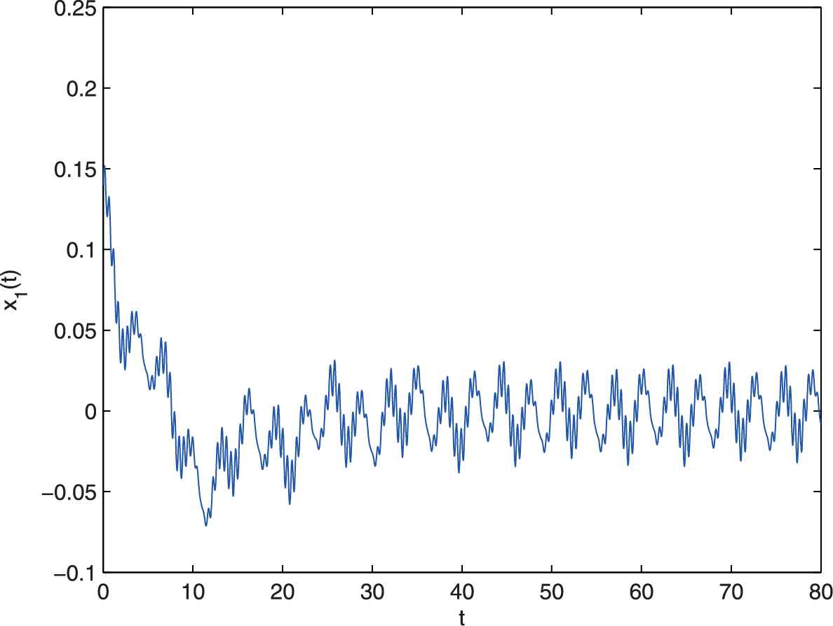
The relation of t and x1.

Figure 2

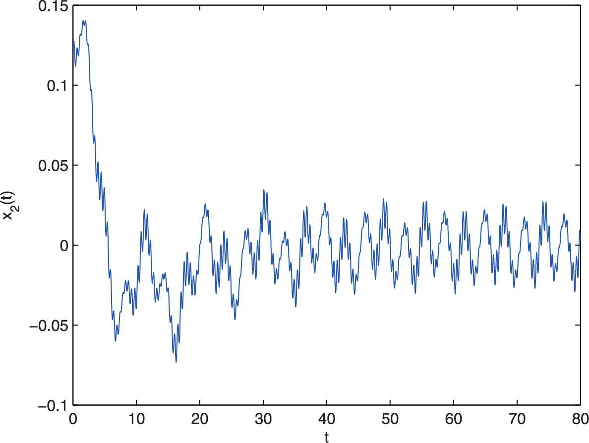
The relation of t and x2.

6. CONCLUSIONS

In this paper, we investigate a class of cellular neural networks with neutral type delays and time-varying leakage delays. Applying the existence of the exponential dichotomy of linear dynamic equations on time scales, a fixed point theorem and the theory of calculus on time scales, we establish a series of sufficient conditions for the existence and exponential stability of almost automorphic solutions for the cellular neural networks with neutral type delays and time-varying leakage delays on time scales. We show that the existence and global exponential stability of almost automorphic solutions for system (1) only depends on time delays ηi(i=1,2,,n) (the delays in the leakage term) and does not depend on time delays τij(i,j=1,2,,n) and σij(i,j=1,2,,n), which implies that the delays in the leakage term do harm to the existence and global exponential stability of almost automorphic solutions. To the best of our knowledge, it is the first time to deal with the almost automorphic solution for cellular neural networks with neutral type delays and time-varying leakage delays on time scales. The idea of this manuscript can be applied directly to investigate a lot of numerous network systems. The theoretical predictions of this manuscript show that under a suitable parameter condition, the cellular neural networks with neutral type delays and leakage delays will display almost automorphic oscillatory phenomenon. In real life, the almost automorphic oscillatory behavior plays an important role in helping us process visual information successfully. It can be effectively applied in predicting the law of brain cell activity, which is useful to serve the diagnosis of diseases. In addition, we know that the quaternion-valued cellular neural networks can be regarded as a generalization of real-valued and complex-valued cellular neural networks. So far, there are very few publications that consider almost automorphic solutions of quaternion-valued cellular neural networks. In the near future, we will focus on this topic.

CONFLICT OF INTEREST

The authors declare that they have no competing interests.

AUTHORS' CONTRIBUTIONS

The study was conceived and designed by Changjin Xu and Maoxin Liao and experiments performed by Peiluan Li and Zixin Liu. All authors read and approved the manuscript.

ACKNOWLEDGMENTS

The work is supported by National Natural Science Foundation of China (No. 61673008), Project of High-level Innovative Talents of Guizhou Province ([2016]5651), Major Research Project of The Innovation Group of The Education Department of Guizhou Province ([2017]039), Innovative Exploration Project of Guizhou University of Finance and Economics ([2017]5736-015), Project of Key Laboratory of Guizhou Province with Financial and Physical Features ([2017]004), Hunan Provincial Key Laboratory of Mathematical Modeling and Analysis in Engineering (Changsha University of Science & Technology)(2018MMAEZD21), University Science and Technology Top Talents Project of Guizhou Province (KY[2018]047), Guizhou University of Finance and Economics (2018XZD01) and Foundation of Science and Technology of Guizhou Province ([2019]1051). The authors would like to thank the referees and the editor for helpful suggestions incorporated into this paper.

REFERENCES

49.F. Ché and Z.B. Nahia, Global attractivity and existence of weighted pseudo almost automorphic solution for GHNNs with delays and variable coefficients, Gulf J. Math., Vol. 1, 2013, pp. 5-24.
51.G.M. N’Guéré, Topics in Almost Automorphy, Springer, New York, 2005.
Journal
International Journal of Computational Intelligence Systems
Volume-Issue
13 - 1
Pages
1 - 11
Publication Date
2020/01/15
ISSN (Online)
1875-6883
ISSN (Print)
1875-6891
DOI
10.2991/ijcis.d.200107.001How to use a DOI?
Copyright
© 2020 The Authors. Published by Atlantis Press SARL.
Open Access
This is an open access article distributed under the CC BY-NC 4.0 license (http://creativecommons.org/licenses/by-nc/4.0/).

Cite this article

TY  - JOUR
AU  - Changjin Xu
AU  - Maoxin Liao
AU  - Peiluan Li
AU  - Zixin Liu
PY  - 2020
DA  - 2020/01/15
TI  - Almost Automorphic Solutions to Cellular Neural Networks With Neutral Type Delays and Leakage Delays on Time Scales
JO  - International Journal of Computational Intelligence Systems
SP  - 1
EP  - 11
VL  - 13
IS  - 1
SN  - 1875-6883
UR  - https://doi.org/10.2991/ijcis.d.200107.001
DO  - 10.2991/ijcis.d.200107.001
ID  - Xu2020
ER  -