
Active and Dynamic Approaches for Clustering Time Dependent Information: Lag Target Time Series Clustering and Multi-Factor Time Series Clustering
- DOI
- 10.2991/jsta.2018.17.3.5How to use a DOI?
- Keywords
- Time Dependent Information; Clustering; Mahalanobis Distance
- Abstract
One of data mining schemes in statistics is clustering panel data such as longitudinal data and time series data. Classical approaches to cluster such time dependent information do not properly count time dependencies among objects we are interested to analyze. In the present study, we propose an approach which takes time dependencies into our consideration by introducing appropriate weight factors with an add-on approach which allows us to measure pairwise distances in multi-dimensional space not just in two dimension. We refer to these approaches LTTC (Lag Target Time Series Clustering) and MFTC (Multi-Factor Time Series Clustering), respectively. These proposed methods in the present study are applicable to any time dependent information from various research areas, and we have applied these methods to state level brain cancer mortality rates in the United States that illustrates the importance of subject methods.
- Copyright
- © 2018, the Authors. Published by Atlantis Press.
- Open Access
- This is an open access article under the CC BY-NC license (http://creativecommons.org/licences/by-nc/4.0/).
1. Introduction
We are living in the world with a flood of information which changes over time, and this time dependent information occupies the main part of BIG DATA that is the current prime topic in data science. There have been several statistical approaches [1] [2] [3] [9] [10] [11] [12] [13] [14] [15] [16] to extract the significant core from time dependent information, and in the present study, we propose new methods to obtain the important essence from the time dependent information by clustering time dependent responses such as time series data and longitudinal data we are commonly faced with to analyze. Figure 1, below describes time dependent information we deal with in Statistics and we focus on time series data and a part of longitudinal data in the present study.
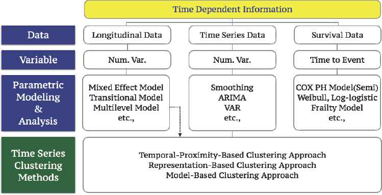
Summary of Time Dependent Information in Statistics.
Classical methods in clustering time dependent information were a sort of a passive approach from a data scientist’s viewpoint, because resulting clusters followed by these methods are deterministic based on the measure of dissimilarity no matter what distance measurements we applied to the data. However, the new methods we are proposing in the present study are active processes to deliver the core information from the massive information we are facing to be analyzed based on our objective of the present study.
In general, we have three different clustering approaches for time dependent information as shown in Figure 1, that is,
- ①
Temporal-Proximity-Based Clustering Approach.
- ②
Representation-Based Clustering Approach.
- ③
Model-Based Clustering Approach.
Our proposed methods are developed in order to accommodate and improve problems inherited from imposing several assumptions in temporal-proximity-based clustering approach. In temporal-proximity-based approach, we assume that there is plenty of information available in each time series object, and only one stream of information is given as a function of time.
But, what if we do not have enough number of observations to use classical time series clustering methods, and what if there exist several significant streams of information in each time series object? Thus, we proceed to introduce two new clustering methods to cover these important cases in temporal-proximity-based approach. Moreover, those classical time series clustering methods do not count actual time dependencies among time series objects and the resulting clusters are usually based on trends and patterns. Hence, we are not able to investigate their actual degree of time dependencies if we use classical time series clustering methods.
2. Motivation
In what follows we discuss the new methods we propose.
2.1. Lag Target Time Series Clustering
The first approach we propose in the current study is “Lag Target Time Series Clustering (LTTC)”. In time series analysis, we usually consider more than 50 observations in each time series objects (responses) as possibly enough information, but this condition is not always satisfied in the real world problem. However, if we take cross lag distances into consideration, we can increase the number of distance measurements considerably.
In Figure 2, below, Xt is the baseline time series object, Yt is a vertical shifted time series object of Xt, and Zt is a preceding index of Xt. Now, which information is more closely related to the baseline time series object, Xt? If we ignore lag-time-dependency between two time series objects, we have
Illustration of the Importance of the Cross Lag Distance.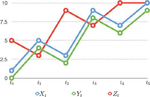
2.2. Multi-Factor Time Series Clustering
The second method we propose in the present study is “Multi-Factor Time Series Clustering (MFTC)”. This method (MFTC) is more meaningful as a more realistic approach to our previously proposed method, LTTC. As we already mentioned in the introduction, one of the general assumptions in classical temporal-proximity-based time series clustering is that there exists only one stream of information in each time series objects. However, usually each time series response consists of several sub-information. For example, daily stock price consists of several sub-information such as opening price, closing price, maximum price, and minimum price, etc. If each sub-information shows different behavior and has a significant impact on the original information, we should take these differences in consideration (sub-information) into our modeling. Also, in health science, survival analysis of patients is a function of time and death is caused by several factors, for example in lung cancer, death was due to smoking, overweight, age, drinking, etc. Thus, we must take these risk factors into consideration in modeling survival analysis. Therefore, when we measure the distance between two time series objects, we now put our ruler in the multi-dimensional space and the degree of dimension is always “the number of factors considered in the study plus one”, because of the time factor. If we just measure cross lag zero distance, it is very trivial as shown in Figure 3. However, when we measure cross lag distances as shown in Figure 4, we have to consider the unit difference between time and other factors and a weight factor which presented in the later section replaces time unit.
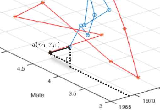
Two-Factor Distance Measurement at the Cross Lag zero.
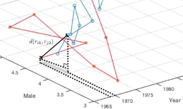
Two-Factor Distance Measurement at the Cross Lag One.
3. An Application of LTTC and MFTC: Brain Cancer Mortality Rates in the United States
In what follows we will apply our methods in some important real data.
3.1. Objective of the Study
There have been various mortality rates statistical models of brain cancer for the entire United States, [4], [5], and [6]. However, we do not have any study done for various regional differences of the brain cancer mortality rates in the United States. We strongly believe that there are signifi-cant regional differences, primarily due to environmental issues such as carbon dioxide emission, the quality of drinking water, etc. that cause death of brain cancer. Thus, our proposed method of analytic clustering procedure based on regional brain cancer mortality rates in the United States is very important.
3.2. Structure of the Data
The data that we are using was collected by the Surveillance, Epidemiology, and End Results (SEER) database which is one of the biggest epidemiological databases in the U.S. and contain U.S. state level mortality rates due to brain cancer from 1969 to 2012. Figure 5, below, shows the structure of the data, with 9 climate regions, 51 states including D.C., and calculated mortality rates for males and females separately. In each state, mt and ft represent the the number of deaths per 100,000 population due to brain cancer at time t( = 1, 2,..., 43) for males and females, respectively.
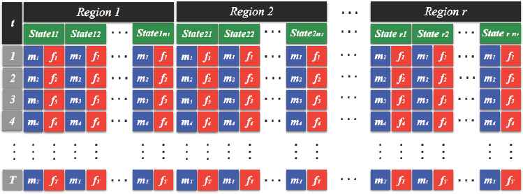
Structure of the Data.
Table 1, below, displays p-values from nonparametric Kruskal-Wallis tests for the hypothesis that the median level of the brain cancer mortality rates of male and female are same in each state of the United States, and calculated p-values in Table 1 suggest for us to consider MFTC method to achieve the objective of the study. [7] [17] [18] For example, the largest p-value we have found in Table 1 is 0.034 for the state of North Dakota and still this p-value is reasonably small enough to decide that the differences between male brain cancer mortality rates and female brain cancer mortality rates are statistically significant, when we set the level of significance, α, at 0.05.
| State | p-value | State | p-value | State | p-value |
|---|---|---|---|---|---|
| IL | 1.56E-14 | NH | 6.40E-06 | FL | 4.85E-14 |
| IN | 1.30E-09 | NJ | 9.38E-14 | GA | 4.42E-13 |
| KY | 1.83E-08 | NY | 1.73E-15 | NC | 9.19E-08 |
| MO | 6.05E-11 | PA | 2.60E-08 | SC | 1.36E-08 |
| OH | 6.45E-15 | RI | 1.32E-05 | VA | 3.01E-11 |
| TN | 7.21E-12 | VT | 2.10E-05 | AZ | 7.56E-10 |
| WV | 1.94E-04 | AK | 6.78E-03 | CO | 5.40E-09 |
| IA | 2.14E-07 | ID | 2.27E-05 | NM | 4.92E-08 |
| MI | 3.59E-11 | OR | 7.62E-11 | UT | 3.74E-06 |
| MN | 2.82E-13 | WA | 7.21E-14 | CA | 1.41E-15 |
| WI | 6.79E-12 | AR | 5.21E-06 | HI | 4.48E-05 |
| CT | 1.24E-11 | KS | 1.60E-10 | NV | 3.56E-09 |
| DE | 7.92E-04 | LA | 7.97E-08 | MT | 3.10E-07 |
| DC | 7.14E-03 | MS | 1.28E-04 | NE | 1.34E-07 |
| ME | 5.58E-07 | OK | 3.70E-10 | ND | 3.40E-02 |
| MD | 2.24E-10 | TX | 7.62E-11 | SD | 6.78E-03 |
| MA | 6.79E-11 | AL | 2.65E-10 | WY | 7.32E-03 |
Comparison Between Male and Female Brain Cancer Mortality Rates.
4. Construction of the Dissimilarity Matrix
Statistical clustering procedures are performed based on the dissimilarity matrix, which is a set of pairwise distances among time series responses. Based on the structure of the data as shown by Figure 5 and using the proposed method MFTC as presented in Table 1, we define pairwise distances as follows.
4.1. Distance at the Cross Lag Zero
First, we define pairwise distances among mortality rates in all U.S. at the cross lag zero. Let
4.2. Distance at the Cross Lag k (k ≥ 1)
We now define kRi, the brain cancer mortality rates in state i after eliminating k rows from the front, and Rj,k, the brain cancer mortality rates in state j after removing k rows from the tail.
4.3. The Dissimilarity Matrix for Clustering
Using the distances we have defined above, we proceed to obtain l layers of the distance matrices as shown in Figure 6, below. In each cross lag distance matrix in Figure 6, di j,k represents the weighted mahalanobis distance between state i and state j at cross lag k.
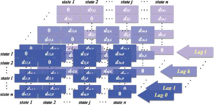
Structure of Distance Matrices.
In order to complete our final dissimilarity matrix for the clustering procedure, we define a weight factor for each layer, which is the ratio of the absolute value of the sample cross-correlation as shown by equation (4.5), and the resulting structure of the weight matrices as displayed in Figure 7. These weight factors take the difference between genders and time dependency between two objects into consideration at the same time properly. That is,
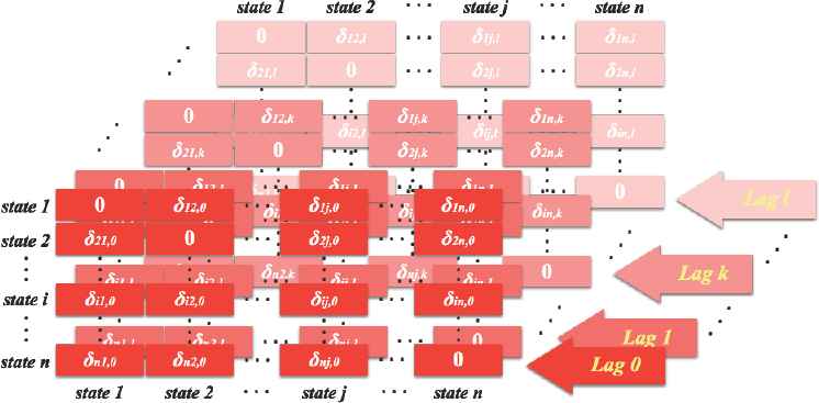
Structure of Weight Matrices.
In each layer in Figure 7, δi j,k denotes the weight for di j,k in Figure 6, that is the weight factor applying to the distance between state i and state j at cross lag k.
Now, we proceed to multiply the distance layers in Figure 6 with the weight layers in Figure 7, and add all the resulting layers to build our final dissimilarity matrix presented in Figure 8 to perform the statistical clustering procedure. At this stage, our main interest lies on the selection of the optimal level of lag distance, and our final dissimilarity matrix is very sensitive to the choice of the optimal level of lag, k.
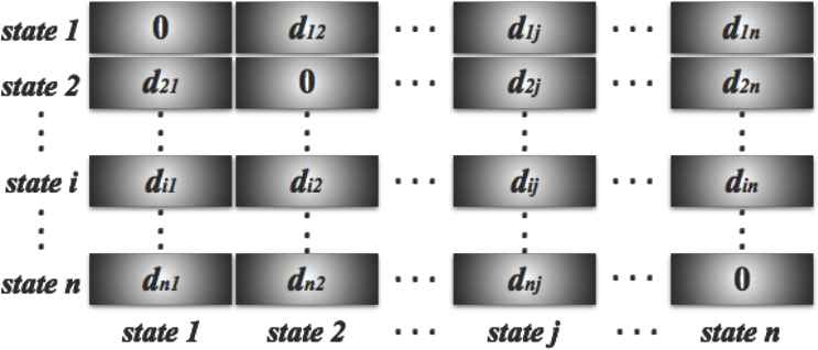
Final Dissimilarity Matrix.
In Figure 8, di j is the final similarity or dissimilarity index between state i and state j. In other words, the sum of weighted cross lag distances between state i and state j.
5. Clustering Procedure
We utilize Ward’s Clustering Method in this section to achieve our resulting clusters. Joe H. Ward, Jr., [21] [22] [23], proposed a general agglomerative hierarchical clustering procedure which is based on minimum variance criterion and it is also called ”Ward’s Minimum Variance Method”. In other words, our final clusters are obtained by minimizing within-cluster variance which is defined by the squared Euclidean distances among clustering objects as shown in equation (5.1), below.
5.1. Clusters Based on Euclidean Distance vs. Mahalanobis Distance
Before we move into our main clustering problem of the brain cancer mortality rates in the U.S., we want to compare the clustering results between Euclidean distance and Mahalanobis distance. Figure 9, presents clustering maps based on Euclidean distance and Mahalanobis distance with the same weight factors described in previous sections. We have four-cluster solution in both clustering maps, and they are almost identical. Only two states stay in different clusters in both maps, and they are Washington state and New Hampshire state. This implies that the covariance between males and females are not significantly large, but this is still statistically significant because the covariance stabilizes the pairwise distances so that we have appropriate level of the effect from using weight factors.
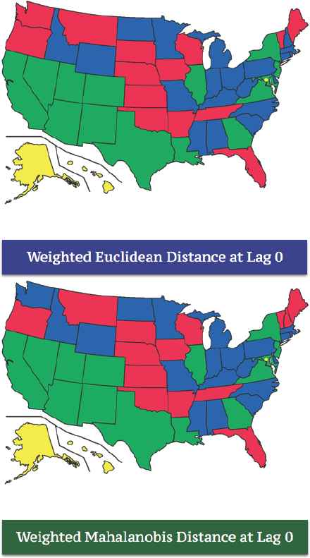
Euclidean Distance vs. Mahalanobis Distance.
5.2. Passive Deterministic Clustering vs. Active Dynamic Clustering
The map at the bottom in Figure 9 delivers the resulting clusters based on our definition of distances from equation (4.1). States in the green cluster are mostly located in the south region of the U.S., and other colored clusters are also determined by the dissimilarity matrix with lag zero which we obtained from the previous sections. With this approach, once we have a dissimilarity matrix where the clustering solution is only determined by the clustering method we want to choose. We refer to this classical approach as “Passive Deterministic Clustering” in this sense.
The algorithm of LTTC is presented in Figure 10, and this procedure is an active and dynamic way to cluster time series responses, because the final cluster solution is the end objective of the present study. Using this method, we first choose our target cluster which consists of time series objects that have similar characteristics, then perform a clustering procedure iteratively by including one more cross lag distance each time until we achieve our target cluster. When we obtain our target cluster, we continue using this procedure again until our target cluster breaks up. If our target cluster breaks up with a dissimilarity matrix with cross lag k distance, our solution to the subject problem is k − 1 lag clustering solution. From this solution, we can see the maximum degree of lag time dependency among time series objects in our target cluster, and minimum lag time dependency in other clusters.
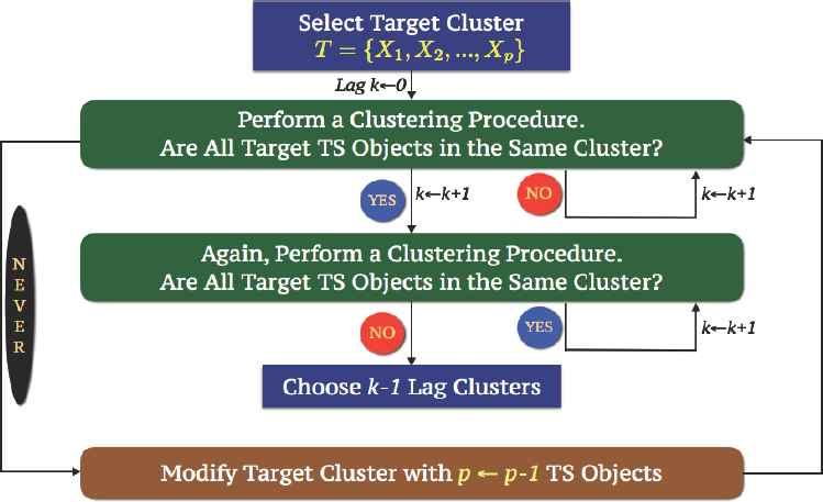
Lag Target Time Series Clustering Algorithm.
5.3. Applying the Proposed Method
Now, we consider that the state of Texas and Florida have similar population characteristics and climate conditions; accordingly our objective of the study is finding the degree of lag time dependency between the two states. As shown in Figure 9, the two states are not in the same cluster when we ignore lag dependency among all of the U.S. states. Therefore, we add lag one distance each time before performing iterative clustering procedures, and then we obtain “Lag 3 Clusters” as our final solution of the subject problem as shown in Figure 11. This implies that brain cancer mortality rates between Florida and Texas have lag 3 time dependency and also we can find other states that have the same lag time dependency with two states as shown in Figure 11.
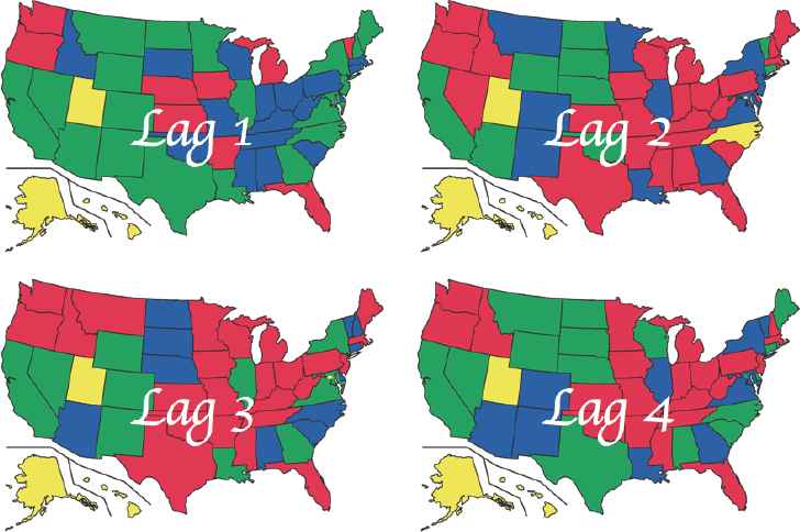
An Example of LTTC Solution.
6. Conclusion
In the present study, we propose an active and dynamic method to cluster time dependent information. The application of MFTC and LTTC, is not confined to cluster ones the same kind of information but also to be able to investigate time dependent relationships among the information from various research areas.
We illustrated the usefulness of the proposed method by clustering an open problem of brain cancer mortality rates in USA. This information is quite important in investigating other risk factors on a regional bases, such as environmental issues that may influence brain cancer deaths.
The proposed active and dynamic procedure is applicable to cluster many important problems in finance, ecology, health sciences, among others. In the present study, we illustrated the effectiveness of the proposed method (procedure) in clustering the brain cancer mortality rates in the USA. Having this information, one can investigate what other effects such as CO2 in the atmosphere, quality of water, etc., may contribute to brain cancer mortality. This procedure can also be applied to cluster breast cancer, lung cancer, prostate cancer, etc.
In finance, clustering the signals (price of a given stock as a function of time) for a given business segment, such as the health industry that consists of a member of stocks is quite important for investing effectively in the subject sector. Using the LTTC and MFTC methods can obtain very important information to portfolio managers for strategic changes in their investment objectives.
References
Cite this article
TY  - JOUR
AU  - Doo Young Kim
AU  - Chris P. Tsokos
PY  - 2018
DA  - 2018/09/30
TI  - Active and Dynamic Approaches for Clustering Time Dependent Information: Lag Target Time Series Clustering and Multi-Factor Time Series Clustering
JO  - Journal of Statistical Theory and Applications
SP  - 462
EP  - 477
VL  - 17
IS  - 3
SN  - 2214-1766
UR  - https://doi.org/10.2991/jsta.2018.17.3.5
DO  - 10.2991/jsta.2018.17.3.5
ID  - Kim2018
ER  -