1. Introduction

One of the most applicable class of models is the class of hierarchical models. It is well-known that the shrinkage estimates play an important role in hierarchical models. In this line, the James-Stein estimators, which combine the partial information of various sources, dominates some other estimators like the ordinary least squares estimators, Stein (1956) and James and Stein (1961). However, the good risk properties of shrinkage estimators make them appealing in many applicable disciplines. Undoubtedly, the basic works of James and Stein on shrinkage estimators became a foundation for the other progressing studies on hierarchical normal models. Stein (1962) described a hierarchical, empirical Bayes interpretation for the shrinkage estimators. Further studies have been done by Efron and Morris (1973), who tried to interpret these kinds of empirical Bayes estimators by several other competing parametric empirical Bayes estimators. Moreover, the homoscedastic (equal subpopulation variances) empirical Bayes interpretation of estimators as well as heteroscedastic (unequal subpopulation variances) ones has motivated various treatments of this problem in hierarchical normal models. For homoscedastic case, we can refer to Baranchik (1970), Strawderman (1971), Brown (1971, 1975) and Berger (1976) among the others, while the heteroscedastic situation have been addressed by a few authors. For more details see Hudson (1974), Xie et al. (2012), Ghoreishi and Meshkani (2014, 2015).

Following considerable work on univariate shrinkage estimators, the multivariate type of James-Stein shrinkage estimators have also been considered for random vectors of dimension r ≥ 3, which either shrink towards the origin vector or another given fixed vector, Lehmann and Casella (1998). James and Stein (1961) showed that the multiple homoscedastic shrinkage estimator of the population mean dominates the corresponding maximum likelihood estimator when r ≥ 3. It means that the multiple James and Stein shrinkage estimator always achieves lower MSE than the corresponding maximum likelihood estimator. Equivalently, the James and Stein multiple estimator makes the maximum likelihood estimator inadmissible when r ≥ 3.

From interpretation point of view, the James and Stein estimator, as an empirical Bayes, is based on the assumption that the population mean is a random vector with an unknown diagonal covariance matrix σ²I and this matrix is estimated from the data itself, Brown (2008), Brown and Greenshtein (2009) and Berger and Strawderman (2009). The main point on this approach is that it is achievable when the random vector of means has a dimension greater than or equal 3 and unfortunately it is not applicable for 2-dimensional random vectors.

The study of James and Stein (1961) on empirical Bayes shrinkage estimators have extended to the case of a general covariance matrix, i.e., where measurements are statistically dependent and may have different variances, see Strawderman (1971) and Bock (1975). They illustrated that the theoretical results on multivariate shrinkage estimator hold when r ≥ 3 and in addition the covariance matrix has the general form σ²D, which is known up to constant σ².

To our knowledge, all results on multivariate homoscedastic James-Stein shrinkage estimators hold for large dimensions r ≥ 3.

The outlines of the paper are:

1. 1)

   We first introduce an alternative class of bivariate shrinkage estimators.

2. 2)

   We study the correlation effect on their performance.

3. 3)

   Since the correlation structure is the biggest challenge in bivariate setting, and this phenomenon can seriously threaten the truth of theoretical results, under some mild assumptions on the model correlations, we show that our proposed estimators have optimal asymptotic properties.

The paper is organized as follows. In Section 2, we review some basic concepts and define necessary notations. The main results of this work, including the risk properties of our bivariate conditional heteroscedastic SURE estimators, are presented in Section 3. We carry out a simple simulation study to evaluate the performance of our proposed bivariate empirical Bayes shrinkage estimators in Section 4 and illustrate the theoretical results for a real data set in Section 5. Necessary technical proofs are given in the appendix.

2. Preliminaries

Let Yi=(Y1iY2i) be the vectors, with 2 × 1 dimension, of normal random variables taken independently at points i = 1,…N. That is

Moreover, The classical conjugate hierarchical model puts a prior of bivariate normal distribution on θ_i

Combination of two assumed model leads us to the following heteroscedastic hierarchical bivariate normal model

where Λ = diag{λ_i} is an unknown 2 × 2 diagonal matrix with positive entries, μ is a 2 × 1 unknown vector and A_is are (potentially) distinct covariance matrices either completely known or will be known by some plug-in robust estimators.

Application of Bayes theorem for model (2.2) gives us the bivariate posterior density

According to this distribution, we consider the posterior means as an alternative class of bivariate shrinkage estimators of θ_i. That is,

As one can see these estimators tend to shrink the sample vectors to the mean vector μ via some coefficients, having important roles to balance observations effect in estimation.

It is straightforward to check that the following relationship holds between the coefficients of estimators (2.3),

for identity matrix I_2×2. Moreover, we have and where a_1i > 0, a_2i > 0 and

It is worth pointing out the following remark concerning our shrinkage estimators.

3. Asymptotic properties of the bivariate SURE estimators

In this section, we show that the proposed bivariate SURE estimators (2.7) have optimal asymptotic properties in comparison with their competitor bivariate estimators. In order to check how well SURE(Λ, μ) function approximates the loss function lN(θi,θˆiΛ,μ) , we have

By rearranging the terms of the above equation, one has

To investigate the risk properties of our bivariate SURE estimators, we need to use Lemma (2.1) in Li(1986). In our setting, it is applicable when the absolute values of UiΛ entries are less than or equal to 1. Hence, the following lemma gives some mild conditions on correlation coefficients to guarantee the framework of Lemma (2.1) in Li(1986). Since the proof is straightforward, it is omitted.

4. Simulation study

In this section, we carry out a simple simulation to study how our bivariate shrinkage estimates perform in comparison with EBMME (Empirical Bayes Method of Moments Estimator) and EBMLE(Empirical Bayes Maximum Likelihood Estimator) bivariate estimators defined below.

• •

  Empirical Bayes method of moment estimators:

  θˆiΛˆEBMME,μˆEBMME=(Ai−1+ΛˆEBMME−1)−1Ai−1Yi+(Ai−1+ΛˆEBMME−1)−1ΛˆEBMME−1μˆEBMME,

  where ΛˆEBMME and μˆEBMME satisfy in

  ∑i=1N(Ai+Λ)−12(Yi−μ)=0,∑i=1N{(Yi−μ)′(Ai+Λ)−1(Yi−μ)−2}=0,

  and the elements of ΛˆEBMME are non-negative.

• •

  Empirical Bayes maximum likelihood estimators:

  θˆiΛˆEBMLE,μˆEBMLE=(Ai−1+ΛˆEBMLE−1)−1Ai−1Yi+(Ai−1+ΛˆEBMLE−1)−1ΛˆEBMLE−1μˆEBMLE,

  where the elements of ΛˆEBMLE and μˆEBMLE are obtained by maximizing the log-likelihood function

  l=cte−12∑i=1Nln{(a1i2+λ1) (a2i2+λ2)−ρi2a1i2a2i2}−∑i=1N12{(a1i2+λ1) (a2i2+λ2)−ρi2a1i2a2i2}{(a2i2+λ2) (Y1i−μ1)2+(a1i2+λ1) (Y2i−μ2)2−2ρia1ia2i(Y1i−μ1) (Y2i−μ2)}.

For our simulation study, we first derive samples for

with marginal distributions a1i2~Unif(1,2) and a2i2~Unif(0.1,1) , and compute the corresponding correlation coefficients under three following scenarios.

• •

  Scenario I: we assume a large correlation coefficient for each i = 1,2,…,N. That is ρi=0.95min(a1i,a2i)max(a1i,a2i) .

• •

  Scenario II: we assume a moderate correlation coefficient, ρi=0.25min(a1i,a2i)max(a1i,a2i) .

• •

  Scenario III: A weak correlation coefficient is considered in this scenario, ρi=0.05min(a1i,a2i)max(a1i,a2i) .

We also assume that θ_i are independently distributed according to

To measure the predictive power of different bivariate shrinkage estimators, we compute the limiting risk limN→∞R(θ,θˆ) for different shrinkage estimators under three scenarios. This process is repeated a large number of times T = 10,000 to obtain an accurate estimate of the average risk for each estimator under three scenarios. Moreover, the sample size N is chosen to be 50 and 200. Table 1 shows the result for various approaches.

Table 1 clearly confirms that although all bivariate shrinkage estimates (SURE, EBMLE and EBMME) have good performance in comparison with the corresponding Oracle risk estimates, our bivariate SURE estimates do better in terms of the risk value under Scenarios (I)-(III). That is, as our theoretical result indicates, the performance of the SURE estimators approaches that of the oracle risk estimators.

5. Application to a real dataset

Educational performance is one of the principle measures for evaluation of an educational center, like a university. It is usually considered through two extreme groups of the students who have either excellent performance (with grade point averages between [17,20]) or poor performance (with grade point averages less than 12) in comparison with the third (moderate) group (with grade point averages between [12,17)). In the following, we use E, M, and P notations which stand for groups of students with Excellent, Moderate, and Poor performances. For a given department indexed by i, let E_i, M_i, and P_i denote the number of students at each group and let n_i denote the number of total students in the corresponding department during the given semester. Whenever it is necessary to consider multiple semesters of educations, such as the two semesters in a given educational year, we will insert other subscripts, and use symbols such as E_ji, M_ji, and P_ji, to denote the number of students with excellent, moderate, and poor performances and total number n_ij for department i (= 1,⋯,N) within semester j (= 1,2).

For data involving N departments over two semesters, we focus on two extreme groups E and P, which are known as educational outcome of each department, Tinto (2010), and assume that

where unobserved parameters p jiE and p jiP are the corresponding proportions of groups E and P with the assumptions of p1iE=p2iE and p1iP=p2iP . Furthermore, the corresponding sample proportions are denoted by pˆ jiE=Ejinji and pˆ jiP=Pjinji . It is obvious that the sample proportions have approximately multivariate normal with vector mean (p jiE,p jiP) , and a covariance matrix that depends on the unknown values p jiE and p jiP .

For our purpose, we are interested in dealing with nearly bivariate normal variables such that a) having variances that depend only on the observed value of n and b) asymptotic performance of bivariate shrinkage estimators are robust with respect to plug-in estimates for the correlation coefficient. From Bartlett (1936, 1947), the standard variance-stabilizing transformations, arcsin En and arcsin Pn may do this goal fairly well for univariate case. However, in our bivariate setting, we prefer to use the transformations

and

For more details on these transformations, see Brown (2008). It is well-known that these transformations have marginal variance-stabilizing properties. That is:

By applying Delta-method for the function arcsin x , it is straightforward to see that the estimated correlation between Y₁ and Y₂ is given by

We would like to note that Lemma (3.1) holds for this correlation and the class of correlations given by (5.1). Furthermore, it is not difficult to numerically verify that the asymptotic performance of our proposed bivariate shrinkage estimators are robust with respect to a general class of the correlation between Y₁ and Y₂

for a positive constant c ≪ n. For more details on marginal transformation of type (5.1), see Brown (2008). If in equation (5.1) we put c = 0, the estimated correlation will be equal to the maximum likelihood estimate of correlation between the sample proportions. In summary, we approximately have

Let’s look at Educational data, Table 2, for 24 departments at University of Qom over the educational year 2014. Our primary focus in this research is to evaluate the students’ performance in the second semester, at each department, when the parameters are estimated based on the first-semester data. Since we use the information of an already-completed educational year, we can then validate our bivariate estimation performance by comparing the estimated values with the real values for the second semester. To evaluate an estimator θˆ based on the transformation Y_2j, we measure the total bivariate sum of squared prediction errors(TSE) defined as

Table 3 summarizes the numerical results of our bivariate shrinkage estimators in comparison with the other competing bivariate shrinkage estimators. The corresponding TSE values are reported. Acceptable performance of our bivariate SURE estimators, among the other estimators, are shown by Table 3. To numerically investigate the robust performance of our bivariate shrinkage estimators, with respect to little changes in correlation coefficient, we present a plot of TSE versus c in (5.1). As Figure 1 illustrates, TSE values of two approaches EBMME and EBMLE always dominate the corresponding values of SURE even for fairly large value of c.

Fig. 1.

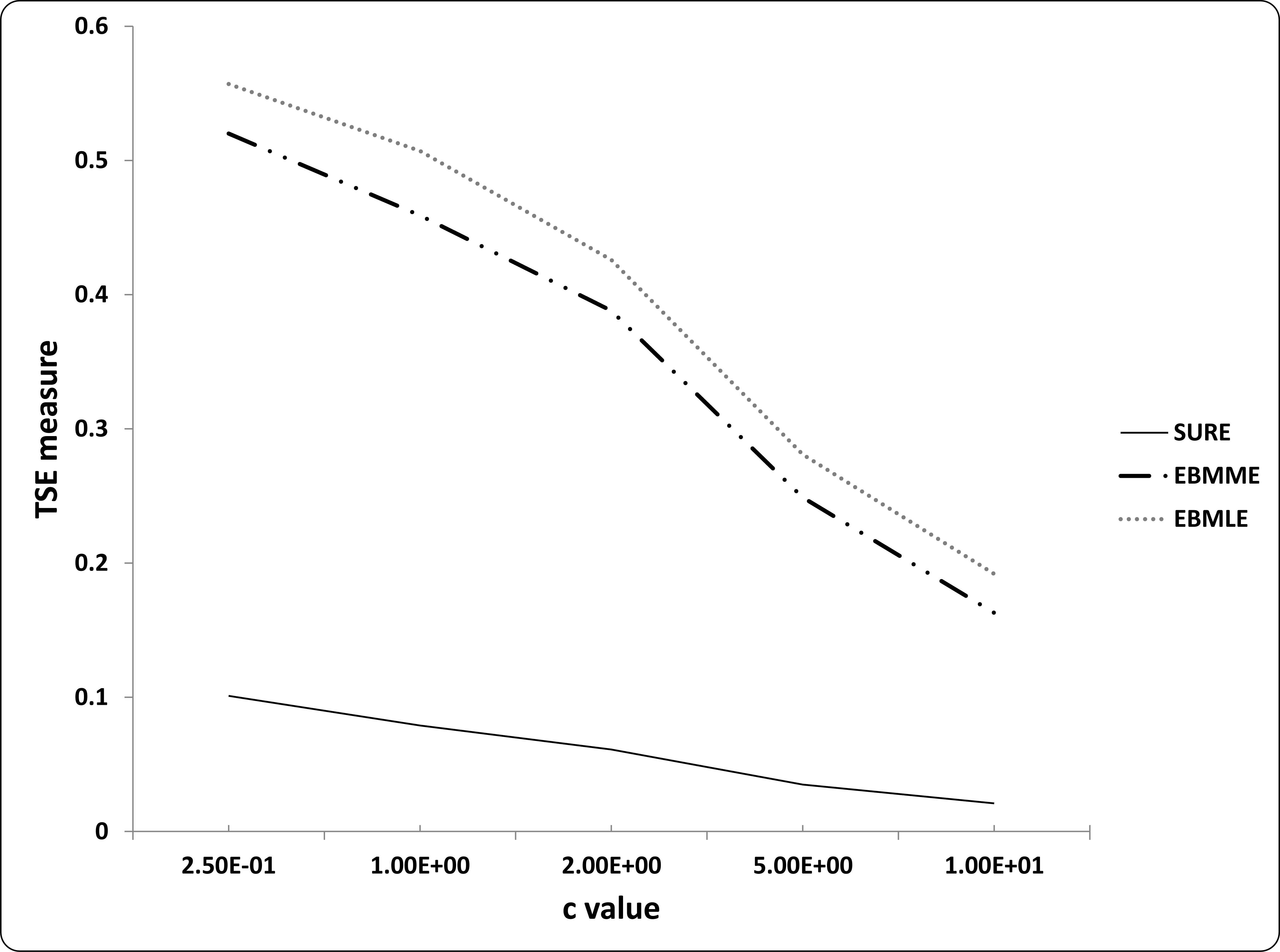
TSE against c values

Acknowledgements

I am grateful to Editor, Associate Editor and three referees for their constructive and insightful comments that helped greatly improve the quality of the paper.