
The Extended Exponential Distribution and Its Applications
- DOI
- 10.2991/jsta.2018.17.2.3How to use a DOI?
- Keywords
- Exponential distribution; Characterization; Generating function; Maximum likelihood; Simulation
- Abstract
We introduce a new three-parameter extension of the exponential distribution called the odd exponentiated half-logistic exponential distribution. Various of its properties including quantile and generating functions, ordinary and incomplete moments, mean residual life, mean inactivity time and some characterizations are investigated. The new density function can be expressed as a linear mixture of exponential densities. The hazard rate function of the new model can be decreasing, increasing or bathtub shaped. The maximum likelihood is used for estimating the model parameters. We prove empirically the flexibility of the new distribution using two real data sets.
- Copyright
- Copyright © 2018, the Authors. Published by Atlantis Press.
- Open Access
- This is an open access article under the CC BY-NC license (http://creativecommons.org/licences/by-nc/4.0/).
1. Introduction
Recently, there are hundreds of generalized distributions which have several applications from biomedical sciences, environmental, engineering, financial, among other fields. These applications have indicated that many data sets following the classical distributions are more often the exception rather than the reality. Hence, the statisticians have been made a significant progress towards the generalization of the classical models and their successful applications in applied areas.
Many authors developed generalizations of the exponential (Ex) distribution. For example, Gupta and Kundu [4] defined the exponentiated Ex (EEx), Nadarajah and Kotz [8] proposed the beta Ex (BEx), Cordeiro et al. [3] pioneered the Kumaraswamy Ex (KEx) as a special case form the Kumaraswamy Weibull distribution, Khan et al. [5] introduced the transmuted generalised Ex (TGEx), Mahdavi and Kundu [6] studied the alpha power Ex (APEx) and Afify et al. [2] studied the Kumaraswamy transmuted Ex (KTEx) distributions.
Afify et al. [1] proposed a wider class of distributions called the odd exponentiated half-logistic-G (OEHL-G) family. The cumulative distribution function (CDF) and probability density function (PDF) of the OEHL-G family are given by
The hazard rate function (HRF) of X is given by
Further information about the OEHL-G can be explored in Afify et al. [1].
In this paper, we propose and study a new three-parameter model called the odd exponentiated half-logistic exponential (OEHLEx) distribution. Based on the OEHL-G family proposed by Afify et al. [1], we construct the new OEHLEx model and give a comprehensive description of some of its mathematical properties. The OEHLEx distribution has some desirable properties like its capability to model monotone and bathtub hazard rates. We show, using two applications, that the OEHLEx distribution can provide better fits than 8 other well-known competing extensions of the Ex distribution.
The rest of the paper is organized as follows. In Section 2, we define the OEHLEx distribution, provide a useful linear representation for its PDF and give some plots for its PDF and HRF. We obtain, in Section 3, some mathematical properties of the proposed distribution including quantile and generating functions, ordinary and incomplete moments, mean residual life, mean inactivity time and some characterization results. In Section 4, we obtain the maximum likelihood estimators (MLEs) of the model parameters and assess the performance of these estimates via a Monte Carlo simulation study. In Section 5, we illustrate the importance of the OEHLEx model using two applications to real data. Finally, in Section 6, we provide some concluding remarks.
2. The OEHLEx distribution
In this section, we define the OEHLEx distribution and provide some plots for its PDF and HRF. By taking G(x;ξ) and g(x;ξ) in (1.2) to be the CDF and PDF of the Ex distribution with PDF and CDF
Then, the PDF of the OEHLEx is given (for x > 0) by
The CDF of the OEHLEx distribution reduces to
Plots of the OEHLEx PDF and HRF for selected parameter values are shown in Figures 1 and 2, respectively. The PDF of the OEHLEx distribution can be symmetric, reversed-J shaped, right skewed or left skewed. The HRF of the OEHLEx distribution can be decreasing, increasing or bathtub shaped.
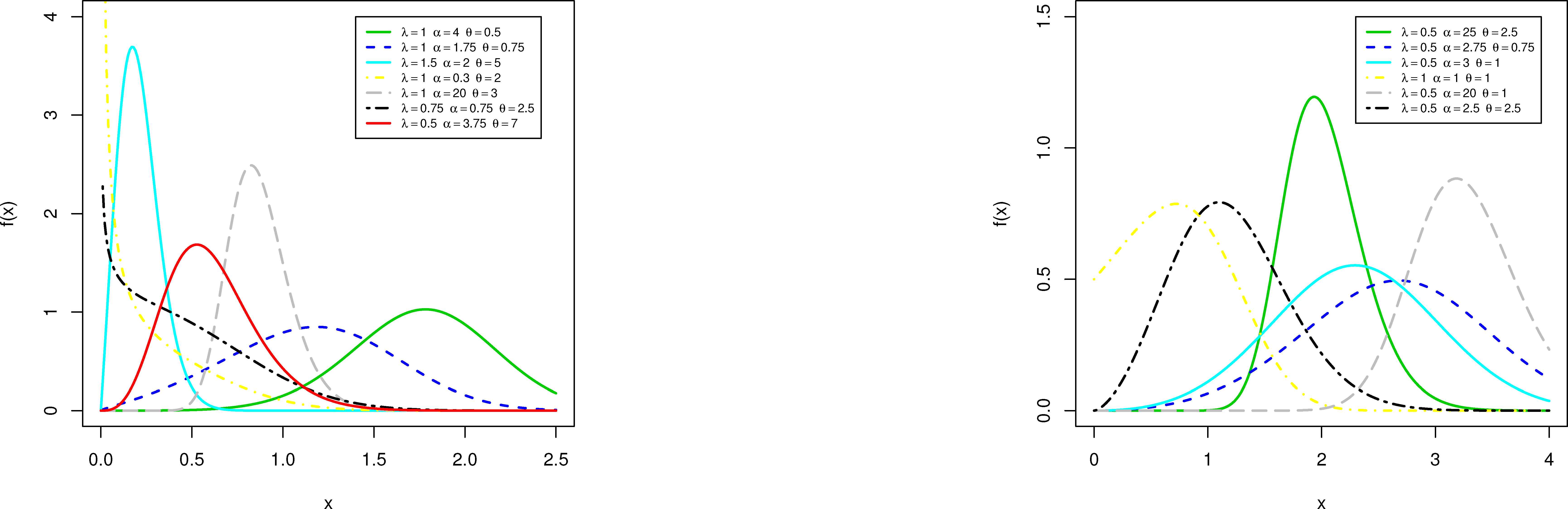
PDF plots of the OEHLEx model for selected parameters values.
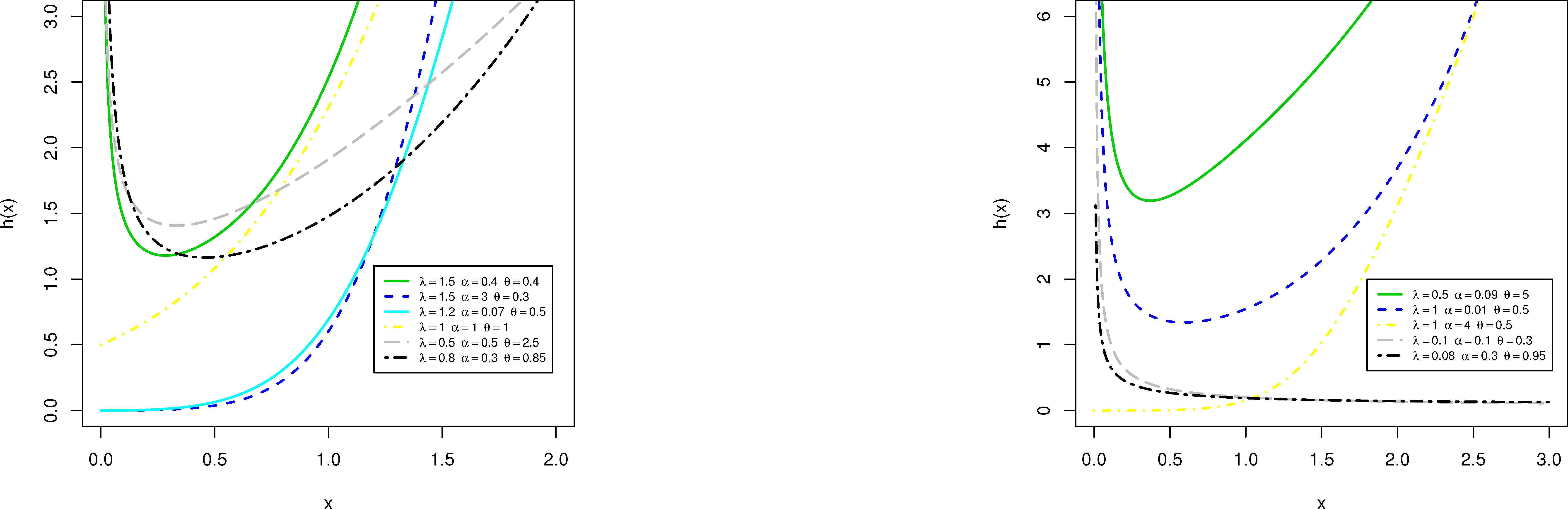
HRF plots of the OEHLEx model for selected parameters values.
Remark 1:
The PDF of the OEHLEx distribution can be expressed as a mixture of Ex densities
Based on Remark 1, several mathematical properties of the OEHLEx distribution can be obtained simply from those properties of the Ex distribution.
Proof.
According to Equation (8) in Afify et al. [1], the PDF of the OEHLEx distribution can be expressed as
Applying the generalized binomial series to (2.5), we obtain
3. Properties and characterization
In this section, we provide some properties of the OEHLEx distribution including quantile and generating functions, ordinary and incomplete moments, mean residual life, mean inactivity time and some characterizations.
Henceforth, let Y be a rv having the Ex distribution in (2.1). Thus, the rth ordinary, incomplete moments and moment generating function (MGF) of Y are given by
3.1. Quantile and generating functions
The quantile function (QF) of the OEHLEx distribution follows, by inverting (2.3), as
Based on (3.1), we can obtain a random sample of size n from (2.3), as Xi = Q(Ui), where Ui∼Uniform(0,1), i = 1,2,…,n.
Using (2.4) and the MGF of Y, we can write the MGF of the OEHLEx model as
3.2. Ordinary and incomplete moments
The sth ordinary moment of X follows from (2.4) as
Using (2.4), the sth incomplete moment of X can be determined as
The first incomplete moment follows from the above equation with s = 1 as
3.3. Mean residual life and mean inactivity time
The life expectancy at age t (for t > 0) or mean residual life (MRL) of X is defined by
By replacing (3.2) in Equation (3.3), the MRL of X can be determined as
The mean inactivity time (MIT) of X is defined (for t > 0) by
By inserting (3.2) in the last equation, the MIT of X follows as
3.4. Characterizations
We will use the following two lemmas to prove the characrterization of the OEHLEx distribution.
Assumption A
Suppose that X is an absolutely continuous rv with CDF F(x) and PDF f(x). We assume E(X) exists and f(x) is differentiable. We assume further
Lemma 1.
If
Proof.
Thus
Differentiating both sides of the above equation, we obtain
By integrating both sides of the above equation, we obtain
Lemma 2.
If
Proof.
Thus
Differentiating both sides of the above equation, we obtain
By integrating both sides of the above equation, we obtain
Theorem 1.
Suppose that X is an absolutely continuous rv with CDF F(x) and PDF f(x). We assume E(X) exists and f(x) is differentiable. We assume further
Then
If and only if
Proof.
We have
Therefore
Suppose
Thus
By Lemma 1, we have
On integrating the above expression, we obtain
Theorem 2.
Suppose that X is an absolutely continuous rv with CDF F(x) and PDF f(x). We assume E(X) exists and f(x) is differentiable. We assume further
Then
Proof.
We have
Therefore
Suppose
Thus
By Lemma 2, we have
On integrating the above expression, we obtain
4. Estimation and simulation
Let X1,…,Xn be a random sample from the OEHLEx distribution with parameters λ, α and θ. Let φ =(λ,α,θ)⊺ be the p × 1 parameter vector. Then, the log-likelihood function for φ is given by
The score vector components,
Setting the nonlinear system of equations Uλ = Uα = Uθ = 0 and solving them simultaneously yields the MLE
Now, we conduct a Monte Carlo simulation study to assess the performance of the MLEs of the unknown parameters for the OEHLEx distribution. The performance of the MLEs is evaluated in terms of their average values and mean squared errors (MSEs). The Mathcad program is used to generate 1000 samples of the OEHLEx distribution for different sample sizes, where n = (20,50,100,150), and for different parameters combinations, where λ =(1,1.5), α =(0.5,0.75,1.5,1.75,3.5) and θ =(0.35,0.5,0.75,1.5,3.5). The average values of estimates and MSEs are provided in Table 1. It is noted, from Table 1, that the MSE decreases as the sample size increases. Thus, the MLE method works very well to estimate the model parameters of the OEHLEx distribution.
| n | Parameters | Average Values | MSEs | ||||||
|---|---|---|---|---|---|---|---|---|---|
| λ | α | θ | λ | α | θ | λ | α | θ | |
| 20 | 1.0 | 0.50 | 0.50 | 0.910 | 0.581 | 0.721 | 0.041 | 0.039 | 0.131 |
| 50 | 1.058 | 0.517 | 0.528 | 0.124 | 0.012 | 1.049 | |||
| 100 | 1.013 | 0.515 | 0.462 | 0.084 | 0.006 | 1.018 | |||
| 150 | 0.966 | 0.516 | 0.631 | 0.044 | 0.004 | 0.135 | |||
| 20 | 1.0 | 0.50 | 1.50 | 1.096 | 0.548 | 1.548 | 0.078 | 0.027 | 0.571 |
| 50 | 1.020 | 0.523 | 1.535 | 0.242 | 0.009 | 0.546 | |||
| 100 | 1.028 | 0.510 | 1.579 | 0.133 | 0.005 | 0.498 | |||
| 150 | 1.043 | 0.503 | 1.546 | 0.062 | 0.003 | 0.415 | |||
| 20 | 1.0 | 0.50 | 3.50 | 1.088 | 0.552 | 3.519 | 0.060 | 0.029 | 0.804 |
| 50 | 1.125 | 0.515 | 3.586 | 0.278 | 0.008 | 2.716 | |||
| 100 | 1.046 | 0.508 | 3.570 | 0.077 | 0.003 | 1.168 | |||
| 150 | 1.025 | 0.503 | 3.538 | 0.039 | 0.002 | 0.731 | |||
| 20 | 1.0 | 1.50 | 0.50 | 1.102 | 1.657 | 0.647 | 0.160 | 0.390 | 0.766 |
| 50 | 1.052 | 1.592 | 0.589 | 0.086 | 0.280 | 0.199 | |||
| 100 | 1.033 | 1.525 | 0.522 | 0.036 | 0.103 | 0.069 | |||
| 150 | 1.019 | 1.510 | 0.515 | 0.021 | 0.060 | 0.043 | |||
| 20 | 1.0 | 3.50 | 0.50 | 1.140 | 4.099 | 0.591 | 0.144 | 4.993 | 0.362 |
| 50 | 1.031 | 3.973 | 0.578 | 0.051 | 2.879 | 0.148 | |||
| 100 | 1.032 | 3.579 | 0.505 | 0.022 | 0.928 | 0.050 | |||
| 150 | 1.027 | 3.515 | 0.495 | 0.014 | 0.473 | 0.030 | |||
| 20 | 1.5 | 0.75 | 0.35 | 1.538 | 0.913 | 0.661 | 0.425 | 0.215 | 0.901 |
| 50 | 1.562 | 0.790 | 0.452 | 0.216 | 0.040 | 0.143 | |||
| 100 | 1.490 | 0.787 | 0.428 | 0.101 | 0.020 | 0.062 | |||
| 150 | 1.482 | 0.772 | 0.403 | 0.059 | 0.012 | 0.034 | |||
| 20 | 1.5 | 0.75 | 0.75 | 1.786 | 0.830 | 0.897 | 0.886 | 0.121 | 1.413 |
| 50 | 1.612 | 0.776 | 0.868 | 0.288 | 0.030 | 0.405 | |||
| 100 | 1.584 | 0.755 | 0.761 | 0.124 | 0.013 | 0.137 | |||
| 150 | 1.558 | 0.757 | 0.751 | 0.066 | 0.009 | 0.089 | |||
| 20 | 1.5 | 1.75 | 0.50 | 1.616 | 1.954 | 0.666 | 0.304 | 0.551 | 0.766 |
| 50 | 1.558 | 1.815 | 0.563 | 0.127 | 0.199 | 0.140 | |||
| 100 | 1.514 | 1.811 | 0.557 | 0.081 | 0.131 | 0.068 | |||
| 150 | 1.502 | 1.785 | 0.550 | 0.064 | 0.110 | 0.051 | |||
Average values of the estimates and the corresponding MSEs for the OEHLEx distribution.
5. Data analysis
In this section, we illustrate the importance of the OEHLEx distribution using two applications to real data. The fits of the OEHLEx distribution will be compared with some competitive models namely: the exponentiated Weibull (EW) Mudholka et al. [7], KEx, KTEx, BEx, gamma (Ga), TGEx, EEx, APEx and Ex distributions, whose PDFs (for x > 0) are given by
EW: f(x) = βλθxβ−1exp(−λxβ) [1 − exp(−λxβ)]θ−1.
KEx: f(x) = abλexp(−λx)[1 − exp(−λx)]a−1 {1 − [1 − exp(−λx)]a}b−1.
KTEx:
BEx:
Ga:
TGEx: f(x) = αλexp(−λx)[1 − exp(−λx)]α−1 × {1 + θ − 2θ [1 − exp(−λx)]α}.
EEx: f(x) = αλexp(−λx)[1 − exp(−λx)]α−1.
APEx:
The parameters of the above densities are all positive real numbers except for the KTEx and TGEx distributions for which |θ| ≤ 1.
The competitive models are compared using some goodness-of-fit criteria including Cramér-Von Mises (W*), Anderson-Darling (A*) and Kolmogorov Smirnov (KS) statistic and its p-value.
The first data set consists of 63 observations of the strengths of 1.5 cm glass fibres, originally obtained by workers at the UK National Physical Laboratory. The data are reported in Smith et al. [10]. The second data set consists of 100 observations of breaking stress of carbon fibres (in Gba) as reported in Nichols and Padgett [9]
Tables 2 and 3 list the W*, A*, KS, its p-value, MLEs and their standard errors (SEs) (in parentheses) for the fitted OEHLEx distribution and other competitive models.
| Distribution | W* | A* | KS | Estimates (SEs) | |||
|---|---|---|---|---|---|---|---|
| OEHLEx (λ,α,θ) |
0.1357 | 0.7698 | 0.1228 (0.2982) |
2.4615 (0.4798) |
1.5777 (0.5047) |
0.0346 (0.0334) |
|
| EW (β,λ,θ) |
0.1999 | 1.1118 | 0.1462 (0.1351) |
7.2846 (1.4868) |
0.0194 (0.0210) |
0.6712 (0.2209) |
|
| KEx (a,b,λ) |
0.2687 | 1.4724 | 0.1615 (0.0749) |
6.8786 (1.1075) |
2553.2883 (5216.1254) |
0.2374 (0.1228) |
|
| KTEx (a,b,θ,λ) |
0.2719 | 1.4899 | 0.1632 (0.0698) |
5.4138 (2.2810) |
386.4380 (515.1351) |
-0.6552 (0.4995) |
0.4231 (0.1449) |
| BEx (a,b,λ) |
0.5687 | 3.1188 | 0.2164 (0.0055) |
17.4493 (3.0818) |
134.5357 (243.8003) |
0.0812 (0.1388) |
|
| Ga (a,b) |
0.5684 | 3.1174 | 0.2164 (0.0055) |
17.4396 (3.0780) |
11.5737 (2.0723) |
||
| TGEx (α,θ,λ) |
0.6992 | 3.8266 | 0.2123 (0.0068) |
31.1539 (11.1417) |
-0.6957 (0.1787) |
2.9097 (0.2579) |
|
| EEx (α,λ) |
0.7862 | 4.2869 | 0.2290 (0.0027) |
31.3495 (9.5201) |
2.6116 (0.2380) |
||
| APEx (α,λ) |
0.6417 | 3.5241 | 0.2235 (0.0037) |
1920499 (23726.92) |
2.0711 (0.0989) |
||
| Ex (λ) |
0.5702 | 3.1270 | 0.4179 (0.0000) |
0.6636 (0.0836) |
|||
The W*, A*, KS (P-value in parentheses) and estimates (SEs in parentheses) for data set I.
| Distribution | W* | A* | KS | Estimates (SEs) | |||
|---|---|---|---|---|---|---|---|
| OEHLEx (λ,α,θ) |
0.0682 | 0.4011 | 0.0639 (0.8088) |
0.2669 (0.1042) |
2.7131 (0.7322) |
2.1000 (1.4127) |
|
| KTEx (a,b,λ,θ) |
0.0685 | 0.4007 | 0.0645 (0.7995) |
2.6891 (3.2607) |
19.4945 (38.547) |
0.227 (0.194) |
-0.6237 (1.7109) |
| KEx (a,b,λ) |
0.0699 | 0.4092 | 0.0647 (0.7969) |
3.2780 (0.8372) |
63.2257 (217.67) |
0.1134 (0.1823) |
|
| EW (β,λ,θ) |
0.0704 | 0.4132 | 0.0645 (0.8003) |
2.4083 (0.5981) |
0.0929 (0.0908) |
1.3175 (0.5905) |
|
| BEx (a,b,λ) |
0.1483 | 0.7589 | 0.0935 (0.3461) |
5.9605 (0.8218) |
34.5462 (61.141) |
0.0615 (0.1021) |
|
| Ga (a,b) |
0.1480 | 0.7572 | 0.0934 (0.3471) |
5.9526 (0.8193) |
2.2708 (0.3261) |
||
| APEx (α,λ) |
0.1843 | 0.9396 | 0.0954 (0.3228) |
34031.74 (12329.98) |
1.0996 (0.0495) |
||
| TGEx (α,λ,θ) |
0.1875 | 0.9581 | 0.0966 (0.3078) |
6.18734 (1.9283) |
1.1019 (0.0947) |
-0.6837 (0.2793) |
|
| EEx (α,λ) |
0.2267 | 0.1859 | 0.1077 (0.1962) |
7.7882 (1.4962) |
1.0132 (0.0875) |
||
| Ex (λ) |
0.1493 | 0.7643 | 0.3206 (0.0000) |
0.3815 (0.0381) |
|||
The W*, A*, KS (P-value in parentheses) and estimates (SEs in parentheses) for data set II.
The figures in these tables show that the OEHLEx distribution has the lowest values for all goodness-of-fit statistics among all fitted distributions.
The histogram of the two data sets, and the estimated CDF, SF and PP plots for the OEHLEx distribution are displayed in Figures 3 and 4, respectively. The plots in Figures 3 and 4 reveal that the OEHLEx distribution has a close fit to both data sets.
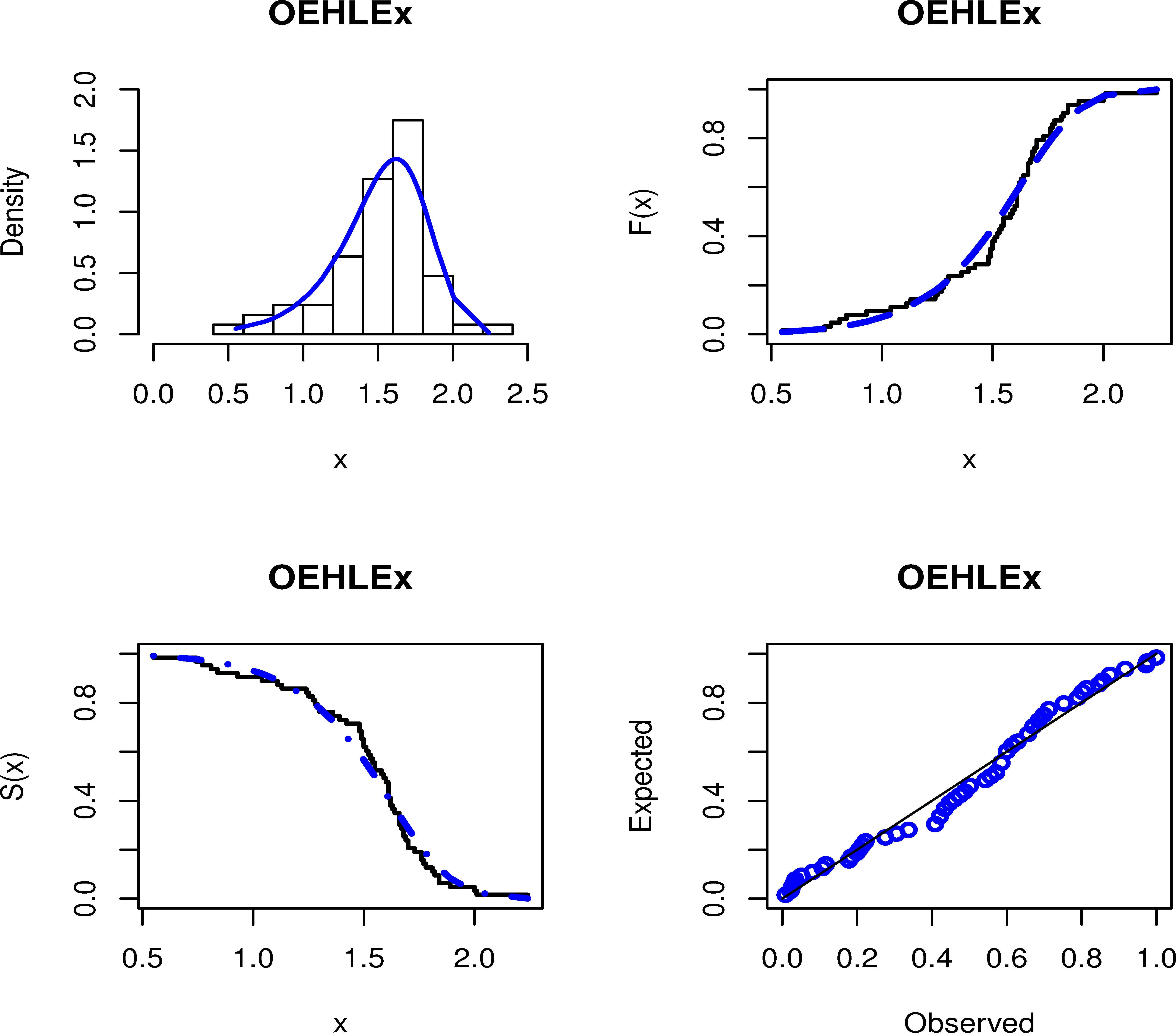
Fitted PDF, CDF, SF and PP plots of the OEHLEx model for data set I.
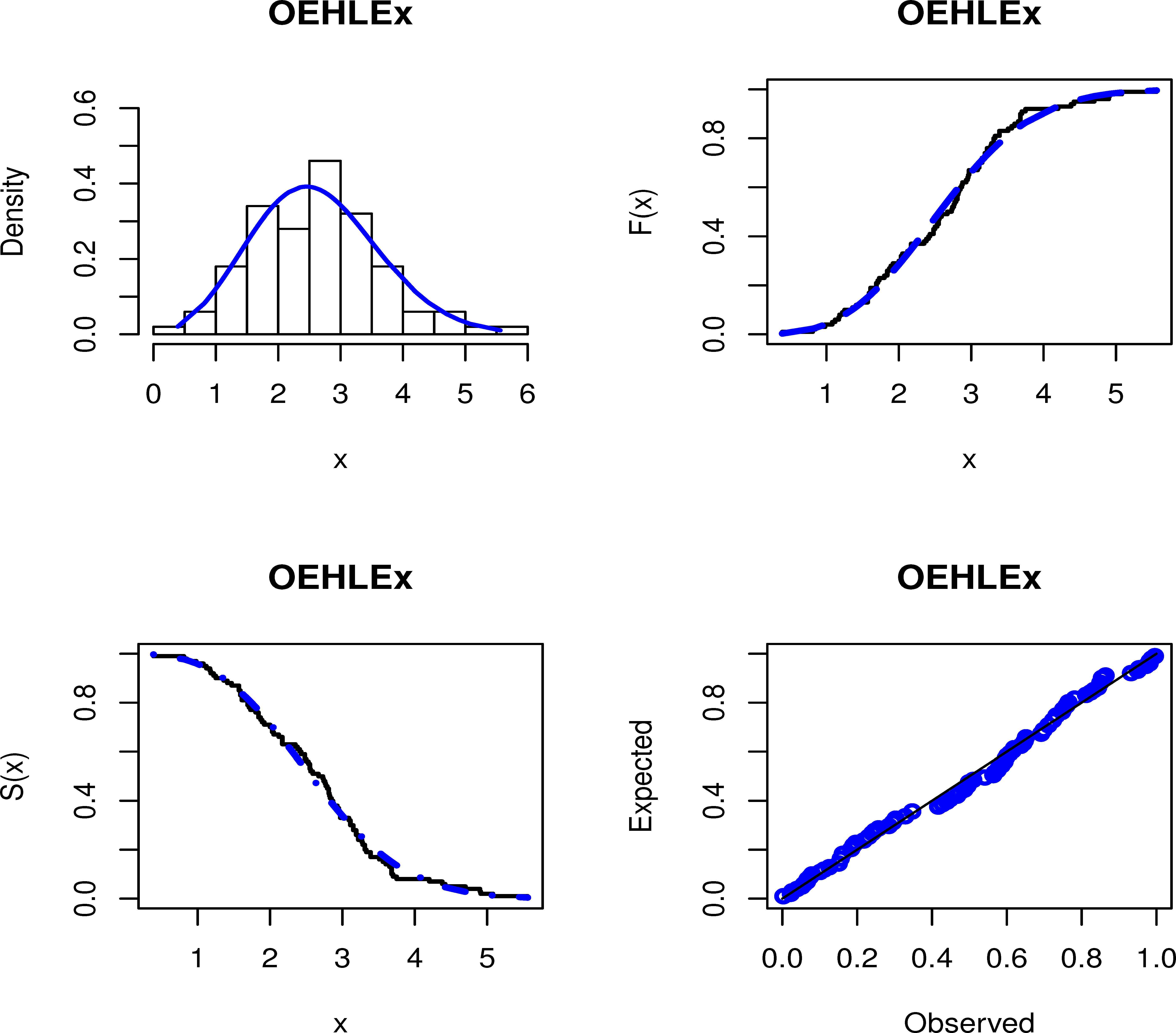
Fitted PDF, CDF, SF and PP plots of the OEHLEx model for data set II.
6. Conclusions
We propose a new odd exponentiated half-logistic exponential (OEHLEx) distribution with two extra shape parameters. The OEHLEx density function can be expressed as a linear mixture of exponential densities. We provide some of its mathematical properties including explicit expressions for the quantile and generating functions, ordinary and incomplete moments, mean residual life and mean inactivity time. The model parameters have been estimated by the maximum likelihood estimation method. We assess the performance of the maximum likelihood estimators via a simulation study. Two applications illustrate that the proposed distribution provides consistently better fits than other competitive models generated using well-known classes.
References
Cite this article
TY  - JOUR
AU  - Ahmed Z. Afify
AU  - Mohamed Zayed
AU  - Mohammad Ahsanullah
PY  - 2018
DA  - 2018/06/30
TI  - The Extended Exponential Distribution and Its Applications
JO  - Journal of Statistical Theory and Applications
SP  - 213
EP  - 229
VL  - 17
IS  - 2
SN  - 2214-1766
UR  - https://doi.org/10.2991/jsta.2018.17.2.3
DO  - 10.2991/jsta.2018.17.2.3
ID  - Afify2018
ER  -