
A Repairable System Supported by Two Spare Units and Serviced by Two Types of Repairers
- DOI
- 10.2991/jsta.d.210611.001How to use a DOI?
- Keywords
- Cold standby; Perfect repair; Patience time; Semi-Markov process; Sojourn time; Busy time
- Abstract
We study a one-unit repairable system, supported by two identical spare units on cold standby, and serviced by two types of repairers. The model applies, for instance, to ANSI (American National Standard Institute) centrifugal pumps in a chemical plant, and hydraulic systems in aviation industry. The failed unit undergoes repair either by an in-house repairer within a random or deterministic patience time, or else by a visiting expert repairer. The expert repairs one or all failed units before leaving, and does so faster but at a higher cost rate than the regular repairer. Four models arise depending on the number of repairs done by the expert and the nature of the patience time. We compare these models based on the limiting availability
- Copyright
- © 2021 The Authors. Published by Atlantis Press B.V.
- Open Access
- This is an open access article distributed under the CC BY-NC 4.0 license (http://creativecommons.org/licenses/by-nc/4.0/).
1. INTRODUCTION
Let us begin with two motivating applications of our general model:
Pumps are of paramount importance in the chemical industry as they are essential to transfer highly corrosive and abrasive chemicals through pipes. The most widely used pump is the ANSI centrifugal pump. Some unique risks associated with chemical plants are abrupt production termination, disastrous plant failure and dangerous environmental interference. These risks result in huge, irrecoverable loses. Therefore, it is critically important to minimize the aforementioned risks by developing a redundant system of multiple, repairable ANSI centrifugal pumps to ensure a very high system availability, while maintaining profitability.
Nowadays, hydraulic systems are widely used in many industries to convert hydraulic energy to mechanical energy. In the aviation industry, hydraulic systems are used in airplanes to operate critical components such as wheel brakes, flight control surfaces, propeller pitch control, landing gear and spoilers, to name but a few. In addition to hydraulic fluid, the main components of the hydraulic system of an airplane are reservoir, pump, valves and actuators. The hydraulic systems of an airplane must be very reliable to minimize any catastrophic risk, such as loss of control, which may threaten many human lives. Hence, it is significantly vital to ensure highly available hydraulic systems and their proper function in an airplane. Maintenance engineers in aviation industry attain this major objective by designing redundant hydraulic systems while maintaining profitability. The redundancy is reached by multiple, repairable hydraulic pumps to provide multiple pressure resources, and multiple, repairable hydraulic actuators to prevent airplane loss of control.
As a theoretical framework for calculating availability and profitability of abovementioned systems, we consider a continuously monitored, one-unit repairable system supported by two other identical units, and serviced by two types of repairers in order to reduce maintenance cost. A regular in-house repairer may have limited maintenance knowledge, but he is paid less per hour and his continual presence eliminates the overhead expense payable to a visiting expert repairer. Generally, the regular repairer can do minor repairs within a given patience time, and is either incapable of performing more complicated repairs, or is unable to do so within the patience time. The visiting expert repairer, on the other hand, can fix any problem with the failed unit, and she performs the repair faster than the regular repairer. However, her hourly charges are comparatively higher, and she must be paid also a trip charge for each visit.
This is how the system operates: Initially, one unit is put on operation and the other two units are on cold standby. Consequently, the system differs from a 1-out-of-3 system. Upon failure of the operating unit, immediately a spare unit is placed on operation, and the failed unit undergoes repair—first by the regular repair person, and if it is not repaired within the patience time
However, the two repairers cannot work simultaneously since the repair facility can accommodate only one repairer at a time. In particular, while a repairer is working on a failed unit, should another unit fail, it must await repair. Also, we assume that the benefit of any partial repair done by the regular repair person is forfeited when the expert takes over the job. We also assume that when repair is complete by either repairer, the repaired unit becomes as good as new.
How long will the expert remain at the repair facility? We consider two possibilities before the expert leaves the system: Either she repairs all failed units while she is visiting, which we call the multiple repair by expert (MRE) policy. Or, she fixes only one failed unit during each visit; and she lets the regular repairer attend to the waiting failed unit(s), if any. This second possibility we call the single repair by expert (SRE) policy.
Depending on the type of patience time—random or deterministic—and the number of repairs done by the expert—single or multiple—four possible models arise: (1) MRE-RPT, (2) SRE-RPT, (3) MRE-DPT and (4) SRE-DPT. We evaluate the performance of these four models in terms of limiting availability
Bieth et al. [2] studies Models (1)–(4), when there is only one spare unit. Assuming exponential life- and repair times, they obtain
We demonstrate that the system with two spare units has higher
The rest of the paper is organized as follows: In Section 2, we give a literature review. In Section 3, we formulate the stochastic behavior of the repairable system as an SMP; and we describe the analytic techniques for deriving the limiting availability and the limiting profit per unit time. In Section 4, we provide detailed analytic derivations for all four repair models. Section 5 compares the four models against those when there is only one spare unit. Finally, Section 6 concludes the paper with a summary and several directions for future research.
2. LITERATURE REVIEW
In this section, we review some latest developments in modeling repairable systems to address various reliability characteristics.
Sarkar and Li [3] considers a one-unit repairable system, supported by
Wang et al. [5] deals with reliability and sensitivity analysis of a repairable system with several operating- and warm standby units, and several unreliable service stations. Failure times and service times are exponentially distributed, and the service station is subject to breakdowns according to a Poisson process. They determine the mean time to failure (MTTF) and system reliability; and study how these characteristics change with the model parameters.
Zhang and Wang [6] studies a cold standby repairable system consisting of two dissimilar components—with Component 1 having priority in use—and one repairman. Component 2 is as good as new after repair, while Component 1 follows a geometric process repair. Assuming exponential life- and repair times, they derive some important reliability indices such as the system availability, reliability, mean time to first failure (MTTFF), rate of occurrence of failure and the probability the repairman remains idle. For Component 1, they determine an optimal replacement policy which minimizes the long-run average cost per unit time.
Yu et al. [7] designs a maintainable cold standby system which minimizes the system cost rate subject to availability constraint. El-Said and El-Sherbeny [8] investigates the cost-benefit analysis of a two-unit cold standby system with two-stage repair with waiting time in between. They use regenerative point processes to obtain time dependent availability, steady-state availability, reliability, MTTF and profit function.
Cui et al. [9] proposes two interval availability indexes for Markov repairable systems which measure the probability that the system is working during a given time window containing either a specified point or an interval. Yi et al. [10] studies a discrete-time semi-Markovian repairable system where the state space of the process includes three subsets—working, changeable and failed. They apply Z-transform to derive reliability, point availability and interval availability. They also discuss for their system the two new reliability measures introduced in [9].
Cha and Finkelstein [11] describes repairable systems in which defects are detected before failure, triggering repair. The system is either perfectly repaired within a time period, and the process renews; or it is not repaired within the time period, causing fatal failure. The authors derive the survival function of these systems assuming exponential time to defect, deterministic time period and arbitrary repair time; though they illustrate the results only under exponential repair time. They also obtain asymptotic survival probability under the assumption of fast repair when distributions are arbitrary.
Tohidi et al. [12] employs cost analysis approach in the redundancy-allocation problem to obtain the optimal number of allocated cold redundant units in a one-unit repairable system. In this system, the main component is put on operation first, and as soon as the failure happens, the redundant component is replaced and the failed unit undergoes repair. They develop a model using continuous-time Markov chain to analyze system reliability assuming that both failure- and repair time are exponentially distributed.
Repairable systems with two types of repairers have not been studied extensively. Kumar et al. [13] studies Model (2) with only one spare unit. They allow an expert to take over the repair only after the patience time of the regular repairer is exhausted without completing the repair, even if the system fails during this time. Sridharan and Mohanavadivu [14] calls in the expert as soon as the patience time is over or the system fails. Although they claim to allow arbitrary life-, repair- and patience time distributions, their results are correct only under exponential life- and exponential repair times, as pointed out in [2]. Sridharan [15] allows a random pre-inspection time for the regular repairer to determine whether he is able to repair a failed unit or not. If he is capable of repairing, he starts the repair; otherwise, the expert is called immediately. Bieth et al. [2] studies Models (1)–(4), when there is only one spare unit. They obtain limiting availability and limiting profit per unit time using the SMP technique under exponential life- and repair times. They also extend the technique to allow arbitrary life- and repair times.
Mahmoud and Moshref [16] allows only one repair person but permits two types of failures and hence two types of repair. They find MTTF, limiting availability and limiting profit using the Laplace transformation technique.
Parashar and Taneja [17] studies a one-unit system backed by a hot standby spare unit in a master–slave relationship. Initially, the master unit is operating and the slave unit is on hot standby. There are three types of failures: minor, major-repairable and major-irreparable (which requires replacement). The regular repairer repairs only minor failures. They claim to derive the system MTTF, steady-state availability and limiting profit per unit time assuming repair- and replacement times are arbitrary but lifetime is exponential; however, no analytic solutions are given. In fact, their theoretical results are valid only under exponential life-, repair- and replacement times.
The papers discussed above utilize the Laplace transform technique to obtain various system reliability indices including, but not limited to, availability, busy periods for the two repairers and profit. None of those papers actually invert the Laplace transform except in the case of exponential distribution. Therefore, we prefer to use the relatively more straightforward and simpler method of SMPs.
3. SYSTEM DESCRIPTION AND MATHEMATICAL FRAMEWORK
For four models discussed in Section 1, we study the system limiting availability and limiting profit per unit time under the following assumptions:
A one-unit system has three identical units. At the very beginning, one unit is put on operation, and the other two spare units remain on cold standby.
There is only one repair facility attended by either the regular or the expert repairer.
Failure of the operating unit is immediately detected; the failed unit is sent for repair, and if a standby unit is available, it is put on operation immediately.
The regular repair person has to finish repair within a maximum allowable patience time
The system fails when all three units are down.
When either the patience time for the regular repair person is over or the system fails, whichever happens first, the expert is called; and she arrives immediately.
Life-, repair- and patience times are exponentially distributed with arbitrary parameters, and are independent of one another. Admittedly, this is a restrictive assumption, which we intend to remove in subsequent research.
When the expert repairer takes over the job, the benefits of partial repair done by the regular repairer is forfeited. In fact, this assumption follows from the previous assumption.
We consider two options for the expert repairer: She may leave the repair facility after repairing all failed units, which is called the MRE model. Or, she may leave the facility after repairing only one failed unit and letting the regular repairer attend to the other failed unit(s), if any. This alternative model is called the SRE model.
We assume a perfect repair policy under which a repaired unit becomes as good as new.
At any time, a unit exhibits one of five possible features:
Figure 1 shows the transitions under SRE and MRE models, along with random variables that determine the sojourn times and transition probabilities.
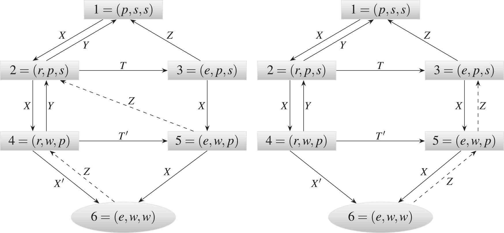
Transition diagrams for SRE (left) and MRE (right) models.
Let us first explain the random variables. Let
Next, let us explain the sojourn times in each state and the transitions out of them. The system starts in State 1 at time
Let
Having obtained
4. LIMITING AVAILABILITY AND LIMITING PROFIT ANALYSIS
In this section, we derive the analytic expressions for the limiting availability
Here, the parameter of an exponential distribution denotes the rate; and its reciprocal denotes the mean. By the memoryless property of an exponential random variable, the future trajectory of the stochastic process depends only on the present state, while the history of the process can be disregarded. Hence, the process, describing each repair model is a SMPs; that is, the system changes states in accordance with a Markov chain, but takes a random amount of time between changes. See [18] for more details on SMP. More specifically, in our models, the embedded discrete-time stochastic process (DTSP) is a Markov chain with a finite state space
The stationary distribution of a Markov chain gives the limiting probability
Moreover, the expected sojourn times in different states are
The following theorem, also quoted from [18], pp. 215–216, gives the proportions of time the SMP spends in the different states.
Theorem 4.1.
For an SMP, if the embedded DTSP is irreducible with stationary probabilities
In the following subsections, for each of the four models, starting from the transition matrix
4.1. Model 1: MRE-RPT
For the MRE-RPT repair model, the embedded DTMC has transition matrix
Solving the system of equations (3), we obtain the stationary distribution as
Substituting the mean sojourn times (4) and the stationary distribution (7) into (5), we can obtain expressions for
Next, the expected length of a cycle satisfies the recursive relation
Solving the system of equations (10), we obtain
Thereafter, we also obtain an explicit expression for
Substituting the expressions for
4.2. Model 2: SRE-RPT
For the SRE-RPT repair model, the embedded DTMC has transition matrix
Solving the system of equations (3), we obtain the stationary distribution as
Substituting the mean sojourn times (4) and the stationary distribution (15) into (5), we can obtain expressions for
To obtain
Substituting the fourth equation into the third in the system of equations (17), we obtain
Substituting (18) into the fourth equation in (17) we obtain
4.3. Model 3: MRE-DPT
For the MRE-DPT repair model, the embedded DTMC has transition matrix
We left unspecified the transition probabilities out of State 4. Let us explain how to obtain them. Write
Thereafter, we have
Substituting the mean sojourn times (4) and stationary distribution (21) into (5), we can obtain expressions for
Moreover,
Using this new expression for
4.4. Model 4: SRE-DPT
Finally, for the SRE-DPT repair model, the embedded DTMC has transition matrix
Substituting the mean sojourn times (4) and stationary distribution (24) into (5), we obtain expressions for
Furthermore,
Using this new expression for
5. COMPARISON OF MODELS
In this section, for some choices of values of the parameters, we compare the four repair models discussed in Section 3 in terms of the limiting availability
Figure 2 depicts
The limiting availability
As
Adding one more spare unit to a system supported by only one spare unit, increases
Suppose that
For our choice of parameter values, the corresponding
Suppose that
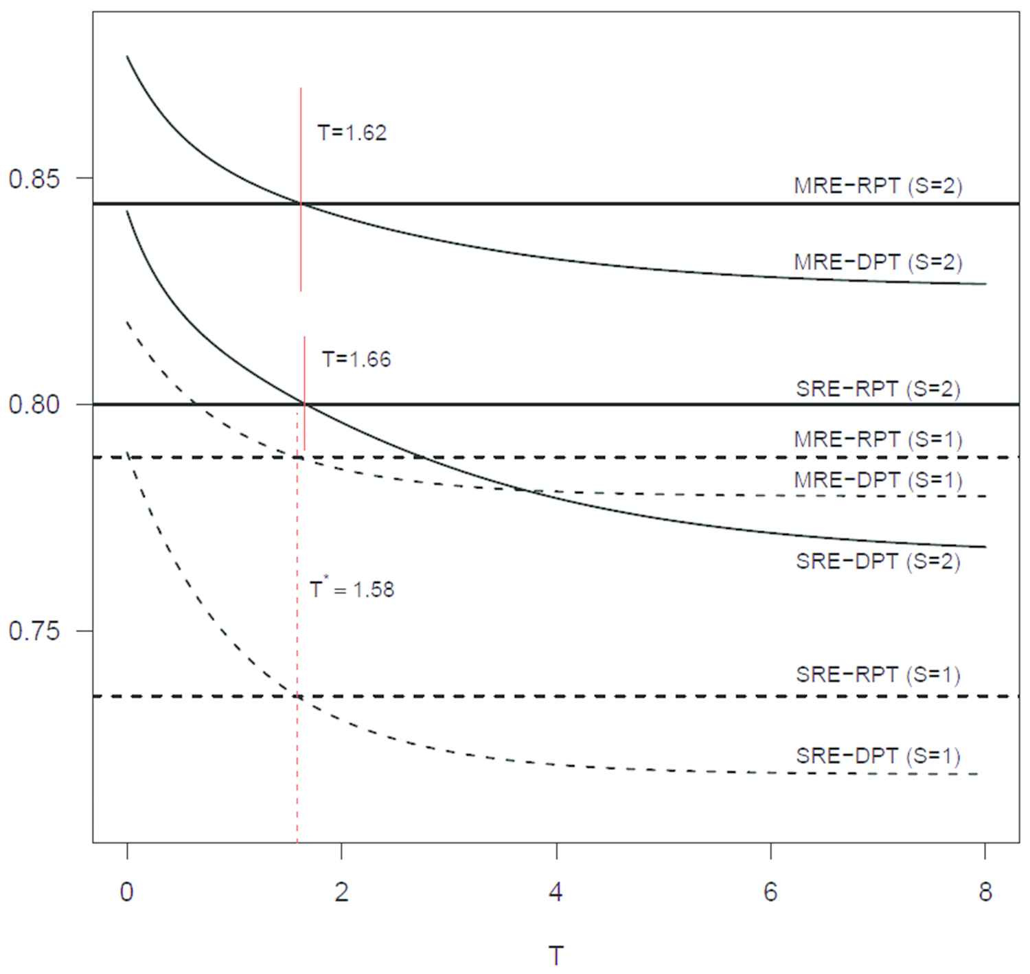
Limiting availability under all repair models for systems with one spare unit (dashed) and two spare units (solid).
Thus, under the limiting availability criterion alone, for the system supported by two spare units, the MRE-DPT model is the best, so long as the patience time is not too long, namely,
Next, we compare the models in terms of the limiting profit per unit time criterion. We assume that the expert repairer completes repair quicker than the regular repairer, but she charges a higher rate; that is,
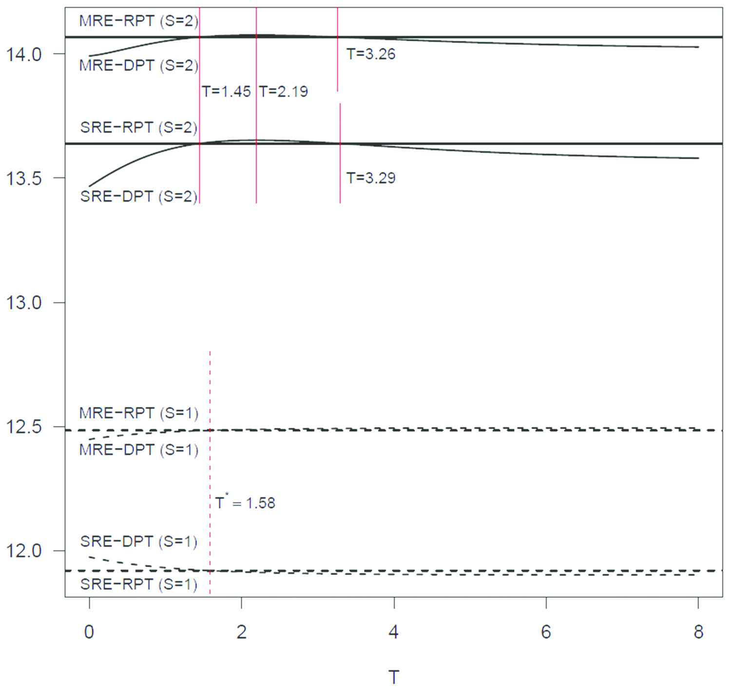
Limiting profit per unit time under all repair models for the systems with one spare unit (dashed) and two spare units (solid).
For our choice of parameter values,we observe the following results:
The limiting profit per unit time
As
Adding one more spare unit to the system backed by only one spare unit, increases
Under
Furthermore, under
Considering both the limiting availability and the limiting profit per unit time criteria simultaneously, we conclude that for any choice of
Although, for our choice of parameter values, it was seen that
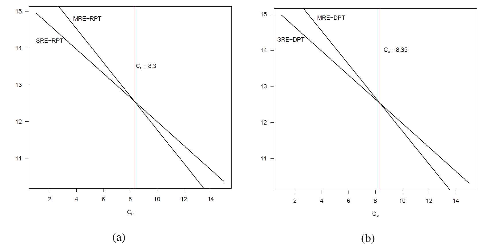
Limiting profit per unit time as a function of
6. CONCLUDING REMARKS
In this paper, we extend [2] by adding another spare unit to a cold standby repairable system consisting of two identical units and serviced by two types of repair persons. In a situation where component lifetime is short and repair time is long, multiple spare units are necessary to improve the reliability characteristics of the system. In this extended set up, we study the limiting availability and the limiting profit per unit time when lifetime and repair times are exponentially distributed. Four possible models arise depending on the number of failed units the expert repairer is allowed to repair during each visit and on the type of patience time for the regular repairer. We derive the limiting availability and limiting profit per unit time for each of the four possible models using SMP, which is much simpler than the Laplace transform technique widely used in the literature. As anticipated, we verify that the system supported by two spare units results in higher
As in [2], in our extended set up also a logistically easier to implement DPT model yields higher
In our motivating examples of ANSI centrifugal pumps in a chemical plant and hydraulically powered components in an airplane, the maintenance engineer can make decisions on how many repairs the expert should do during each visit and how much patience time should be given the regular repairer to ensure higher limiting availability and limiting profit per unit time. Such informed decisions will minimize substantial risks associated with the chemical plant and airplane.
We identify several directions of future research:
For the purpose of building the repairable models, we have assumed life- and repair times to be exponential. Relaxing these assumptions, though desirable, may prove to be challenging since the stochastic process will no longer be an SMP.
We assumed that there is only one repair facility that allows only one repairer to work at a time. It will be advantageous to employ two repair facilities so that both repairers can work at the same time. Under this assumption, the transition diagram becomes more complicated involving more states. In addition, the Markovian property fails under the DPT policy, since the transition out of some states may depend not only on the current state but also on the history of the process.
We assumed that the units are identical. It is desirable to study a more realistic system involving nonidentical units with different life- and repair rates. In particular, we must determine which unit should be put on operation and which on repair whenever there are multiple such units.
CONFLICTS OF INTEREST
The authors declare that there is no conflict of interest.
AUTHORS' CONTRIBUTIONS
Both authors have contributed equally to problem identification, mathematical development, computations, and conclusions.
Funding Statement
This research received no specific grant from any funding agency in the public, commercial, or nonprofit sectors.
ACKNOWLEDGMENT
The authors are grateful to the editor-in-chief and the anonymous referees for their helpful suggestions.
REFERENCES
Cite this article
TY  - JOUR
AU  - Vahid Andalib
AU  - Jyotirmoy Sarkar
PY  - 2021
DA  - 2021/07/10
TI  - A Repairable System Supported by Two Spare Units and Serviced by Two Types of Repairers
JO  - Journal of Statistical Theory and Applications
SP  - 180
EP  - 192
VL  - 20
IS  - 2
SN  - 2214-1766
UR  - https://doi.org/10.2991/jsta.d.210611.001
DO  - 10.2991/jsta.d.210611.001
ID  - Andalib2021
ER  -