
On Finite 3-Component Mixture of Rayleigh Distributions: A Classical Look
- DOI
- 10.2991/jsta.d.210616.001How to use a DOI?
- Keywords
- Mixture distribution; Maximum likelihood estimation; Statistical properties; Entropies; Inequality measures; Order statistics
- Abstract
In this study, we have discussed various statistical properties for 3-component mixture of Rayleigh distributions. Here initially, the main properties of mixture distributions are presented and analyzed. Second, some of the famous entropies, measures of inequality are also discussed. Also, the statistical properties of the density functions of rth-, 1st- and nth-order statistics are derived. Moreover, the parameters estimation of the considered mixture model under the maximum likelihood (ML) estimation is also performed using censored and complete data scheme. Finally, the results on ML estimation are also computed via Monte Carlo simulation study and as well as by using a real-life data set.
- Copyright
- © 2021 The Authors. Published by Atlantis Press B.V.
- Open Access
- This is an open access article distributed under the CC BY-NC 4.0 license (http://creativecommons.org/licenses/by-nc/4.0/).
1. INTRODUCTION
Mixture of distributions is arising naturally and discussed where a statistical population has more than two sub populations. In many applicable areas, the mixture representations have been compensated excessive care. However, the mixture of distribution that rises with a grouping of different distributions is said to be a mixture component, and the probabilities (weights) which are related to each of the component are known as the mixture weights.
In different practical situations, several authors have worked on the mixture modeling. Mostly, in the biology the direct applications of the mixture models are discussed by Bhattacharya [1] and by Gregor [2], in the medicine are presented by Chivers [3] and by Burekhardt [4], in the social sciences are observed by Harris [5], in an economics are mentioned by Jedidi et al. [6], in the reliability and survival are analyzed by Sultan et al. [7], in the life testing are suggested by Shawky and Bakoban [8], in the industrial engineering are observed by Ali et al. [9].
This study plan to develop a 3-component mixture of Rayleigh distributions for an effective modeling of time-to-failure data. Let consider a variable of interest y which follows a mixture distribution having
The cdf
2. STATISTICAL PROPERTIES
Here, we derive computable representations of some statistical properties associated with the 3-component mixture of Rayleigh distributions having pdf given in (1).
2.1. rth Moments about Origin
The
2.2. Mean and Variance
The mean and variance of the considered mixture distributions are as follows:
2.3. hth-Order Negative Moments
If we replaced
2.4. Factorial Moments
If we replaced
2.5. Quantile Function
The quantile function for a
2.6. Median
To solve the below mentioned Equation (10) for y, we obtain the median as follows:
2.7. Mode
To resolve the below mentioned Equation (11) for y, we obtain the mode as follows:
The numerical results of mean, median, mode, variance and coefficient of skewness for various choices of
| Mean | Variance | Median | Mode | Skewness | |
|---|---|---|---|---|---|
| 13, 14, 15, 0.1, 0.2 | 18.2984 | 91.6779 | 17.1902 | 14.5176 | 0.075906 |
| 13, 14, 15, 0.2, 0.3 | 17.9224 | 88.0297 | 16.837 | 14.1885 | 0.0759013 |
| 13, 14, 15, 0.3, 0.4 | 17.5464 | 84.3814 | 16.4837 | 13.8928 | 0.0759134 |
| 13, 14, 15, 0.4, 0.5 | 17.1704 | 80.7332 | 16.1305 | 13.6268 | 0.0759086 |
| 15, 14, 13, 0.2, 0.1 | 16.9197 | 78.5014 | 15.895 | 13.3907 | 0.0759137 |
| 16, 15, 14, 0.3, 0.2 | 18.549 | 94.339 | 17.4257 | 14.6759 | 0.0759014 |
| 17, 16, 15, 0.4, 0.3 | 20.1784 | 111.55 | 18.9563 | 15.9914 | 0.0759112 |
| 18, 17, 16, 0.5, 0.4 | 21.8077 | 130.135 | 20.4869 | 17.3345 | 0.0759137 |
| 12, 11, 10, 0.4, 0.2 | 13.7865 | 52.277 | 12.9515 | 10.8186 | 0.0759095 |
| 14, 13, 12, 0.4, 0.2 | 16.2931 | 72.8788 | 15.3063 | 12.8464 | 0.195787 |
| 16, 15, 14, 0.4, 0.2 | 18.7997 | 96.9142 | 17.6612 | 14.8668 | 0.179804 |
| 18, 17, 16, 0.4, 0.2 | 21.3063 | 124.383 | 20.016 | 16.8825 | 0.167591 |
Mean, variance, median, mode and skewness.
It is revealed that the distribution of the 3-component mixture of Rayleigh distributions is positively skewed because the value of mean is greater than median and SK > 0 (cf. Table 1). As the values of
3. RELIABILITY PROPERTIES OF THE PROPOSED MIXTURE DISTRIBUTIONS
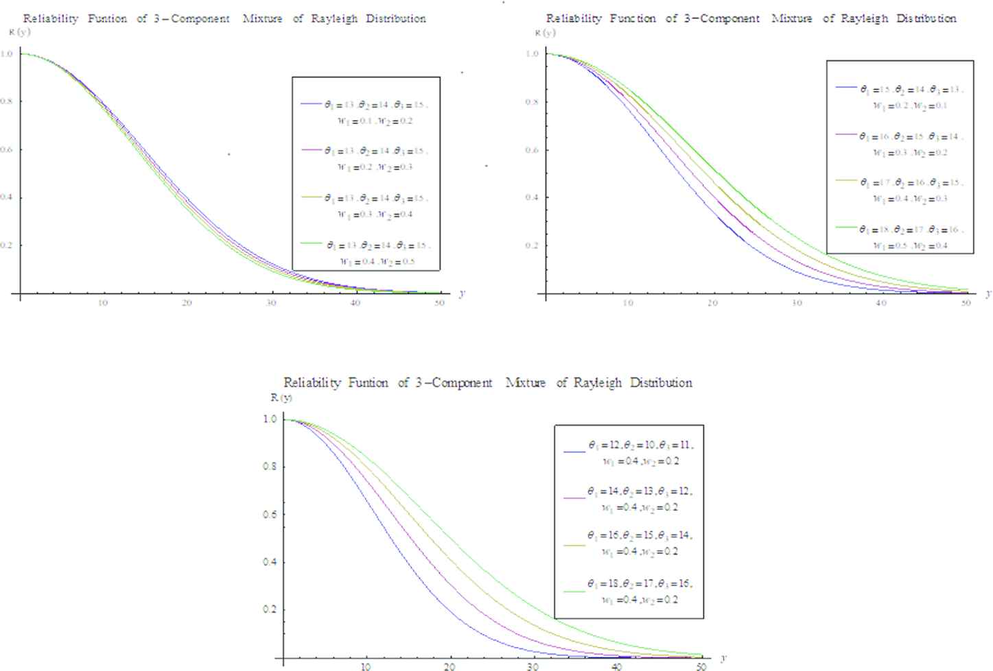
3.1. Reliability Function
The reliability function of the proposed mixture distributions is given as follows:
The graphical presentation of the reliability function for proposed mixture distributions is as follows:
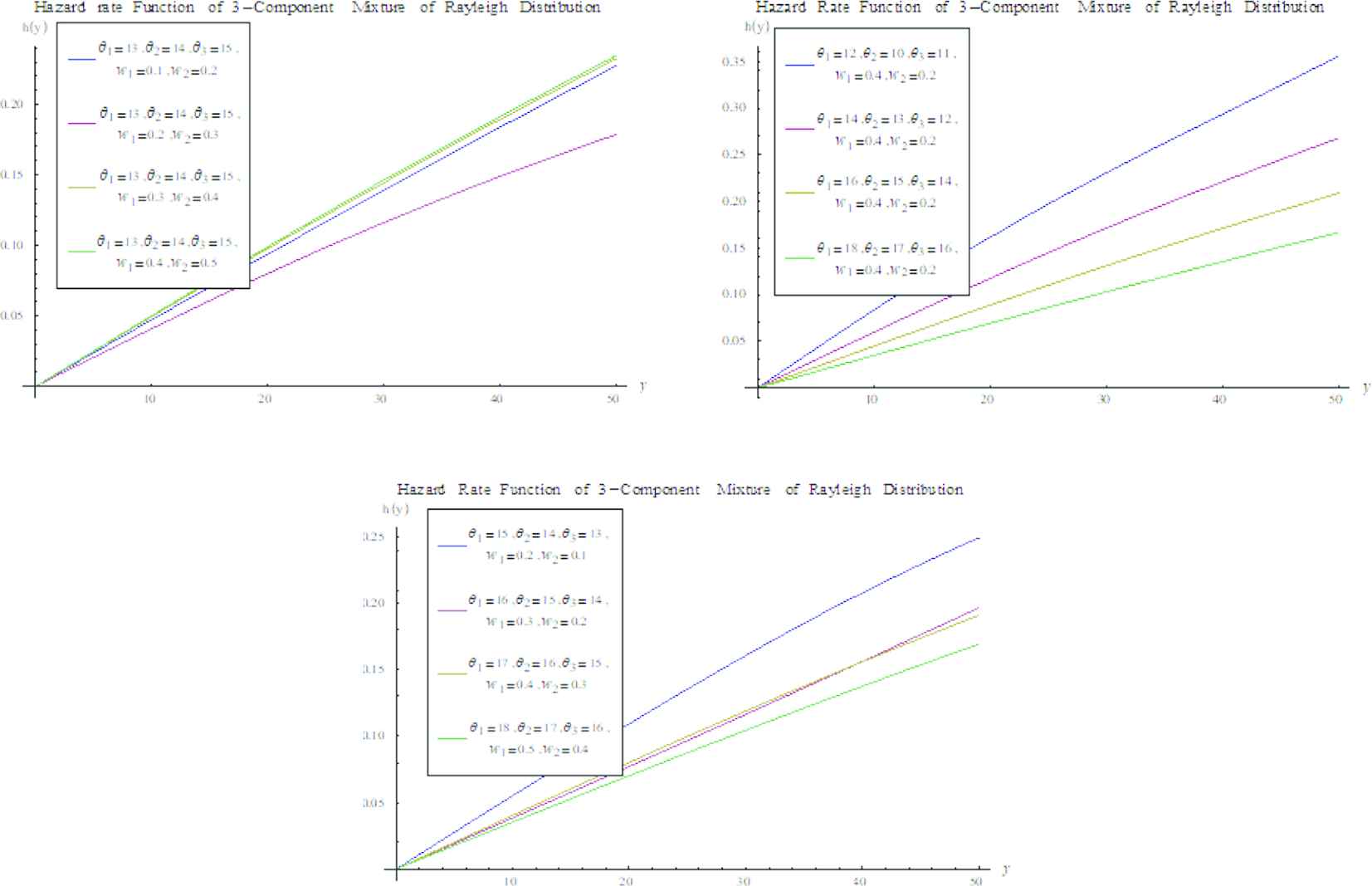
3.2. Hazard Rate Function
The hazard rate function for proposed mixture distributions is as follows:
The graphical performance of the hazard rate function for proposed mixture distributions is given as follows:
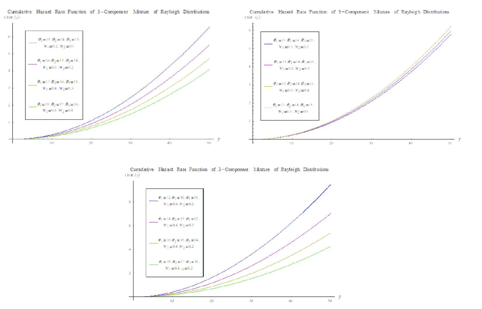
3.3. Cumulative Hazard Rate Function
The cumulative hazard rate (CHR) function for proposed mixture distributions is defined as follows:
The graphical performance of the CHR function for proposed mixture distributions is shown as follows:
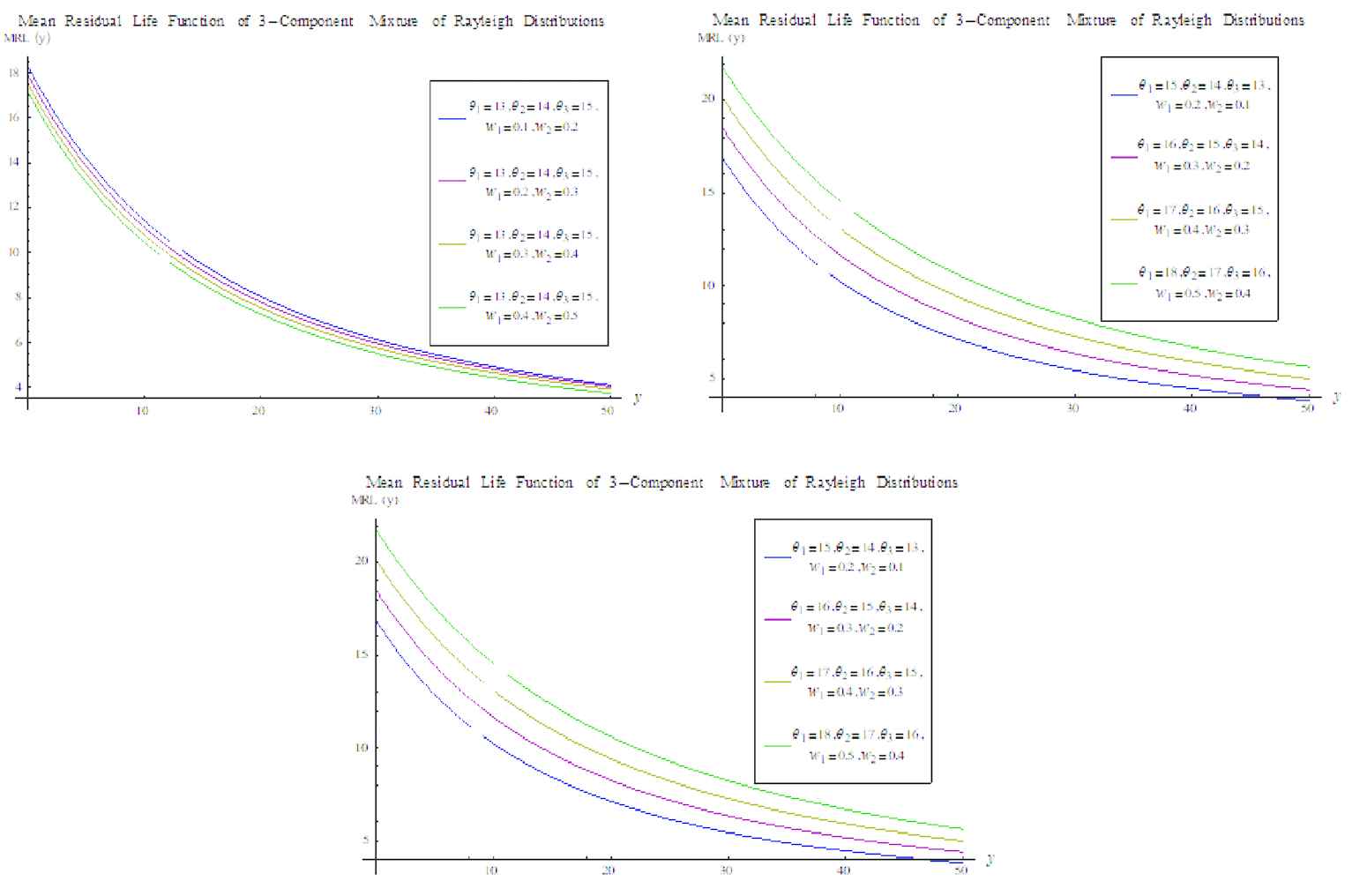
3.4. Mean Residual Life Function
The mean residual life (MRL) function for proposed mixture distributions is written as follows:
The graphical performance of the MRL function for proposed mixture distributions is shown as follows:
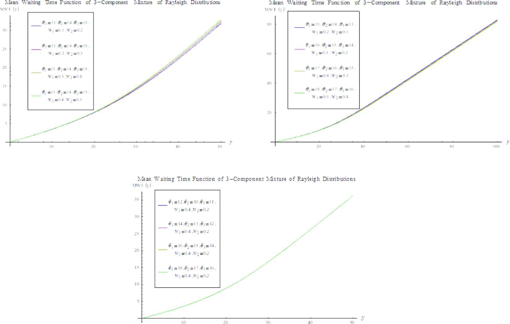
3.5. Mean Waiting Time Function
The mean waiting time (MWT) function for proposed mixture distributions is defined as follows:
The graphical presentation of the MWT function for proposed mixture distributions is shown as follows:
4. STATISTICAL FUNCTIONS
The different statistical functions such as moment generating function
5. MEASURES OF INEQUALITY
In this section, we have considered various measures of inequality such as Gini index (G), Lorenz curve
After substitution the values in (36), the simplified Zenga index is as follows:
6. ENTROPIES
The entropy is used as measure of uncertainty in various applied fields of science and engineering. The various type of entropy such as Shannon's entropy
7. DISTRIBUTIONS OF ORDER STATISTICS
In this section, we have provided the different function of order statistics such as kth, 1st and nth for proposed mixture distribution. The mean and variance of considered order statistics are also presented.
7.1. The kth-Order Statistic
The pdf of
After substitution in Equation (37), we get
7.2. The 1st-Order Statistic
Placing
7.3. The nth-Order Statistic
Replacing
7.4. rth Moments about Origin of 1st- Order Statistic
The
The mean and variance of 1st-order statistic are obtained as follows:
7.5. rth Moments about Origin of nth- Order Statistic
The
The mean and variance of the
8. ESTIMATION OF PARAMETERS
The ML method is used to estimate the unknown parameters of the proposed mixture distribution under type-I censored and complete sampling situations. The ML estimation under type-I censored and complete sampling situations are given below:
8.1. The Likelihood Function
The likelihood function for suggested mixture distribution under type-I censoring is written as follows:
After simplifying the Equation (47), we get
8.2. ML Estimators and Their Variances for Censored Data
The ML estimators for
It is tough to find out the closed form for the ML estimators. The normal equations do not have explicit solutions and they have to be obtained numerically. The Mathematica (Wolfram [10]) software is used to find the ML estimates (MLEs) of
The simplest large sample approach is to assume that the MLE
8.3. ML Estimators and their Variances for Complete Data
All the censored observations become uncensored if t approaches to
9. MONTE CARLO SIMULATION
In this section, we have used Monte Carlo simulation to find the MLEs and MLVs for the proposed mixture distribution. Through the following steps, we obtained the MLEs and MLVs, as follows:
First we generate
A censored sample is selected at a fixed
The Steps 1 and 2 are repeated 1000 times for all selected choices of parameters.
To find the MLEs and MLVs of
The abovementioned Steps 1–4 used for different sample size n = 50, 100, 200, 500, parameters values
From Tables 2 and 3, if
| 24 | 50 | 11.80089 | 14.61541 | 15.01973 | 0.311001 | 0.450384 |
| 24 | 100 | 12.14090 | 14.47142 | 15.79121 | 0.309475 | 0.459040 |
| 24 | 200 | 12.32481 | 14.41900 | 15.71900 | 0.306542 | 0.471284 |
| 24 | 500 | 12.64047 | 14.30591 | 15.49235 | 0.305908 | 0.483244 |
| 32 | 50 | 12.30870 | 14.50639 | 15.28540 | 0.307408 | 0.473077 |
| 32 | 100 | 12.572412 | 14.32247 | 15.64205 | 0.305157 | 0.482970 |
| 32 | 200 | 12.70826 | 14.24910 | 15.39890 | 0.303980 | 0.489530 |
| 32 | 500 | 12.81997 | 14.11887 | 15.19401 | 0.302209 | 0.496001 |
The MLEs values of the proposed mixture distribution for
| 24 | 50 | 14.95881 | 15.60520 | 14.95971 | 0.442387 | 0.314019 |
| 24 | 100 | 15.20851 | 15.47148 | 14.84121 | 0.459401 | 0.311701 |
| 24 | 200 | 15.32170 | 15.40986 | 14.55412 | 0.470451 | 0.310951 |
| 24 | 500 | 15.71638 | 15.29501 | 14.42015 | 0.482201 | 0.308541 |
| 32 | 50 | 15.41810 | 15.55680 | 14.21510 | 0.461050 | 0.309451 |
| 32 | 100 | 15.54207 | 15.39238 | 14.74209 | 0.485094 | 0.306105 |
| 32 | 200 | 15.70844 | 15.25910 | 14.43770 | 0.489451 | 0.304404 |
| 32 | 500 | 15.85159 | 15.13786 | 14.21241 | 0.495001 | 0.302199 |
The MLEs values of the proposed mixture distribution for
From Tables 4 and 5, it is revealed that the
| 50 | 12.88630 | 13.89810 | 14.68280 | 0.30000 | 0.50000 |
| 100 | 12.90350 | 13.93310 | 14.90500 | 0.30000 | 0.50000 |
| 200 | 12.96220 | 13.97070 | 14.94290 | 0.30000 | 0.50000 |
| 500 | 12.96660 | 13.99730 | 14.99860 | 0.30000 | 0.50000 |
The MLEs values of the proposed mixture distribution for
| 50 | 15.91150 | 14.93810 | 13.87220 | 0.50000 | 0.30000 |
| 100 | 15.94880 | 14.95030 | 13.92910 | 0.50000 | 0.30000 |
| 200 | 15.95560 | 14.97220 | 13.98150 | 0.50000 | 0.30000 |
| 500 | 15.98630 | 14.98730 | 13.99820 | 0.50000 | 0.30000 |
The MLEs values of the proposed mixture distribution for
10. APPLICATION BASED ON REAL DATA SET
In this section, we present the real-life application of the proposed mixture distribution based on three components, i.e., Transmitter Tube (V805), Transmitter Tube and Indicator Tube (V600) related to the aircraft (cf. Davis [11]). Davis [11] showed that the distribution of these components is exponential. For an exponential random data
The MLEs and MLVs are shown in Table 6.
| MLEs | 600 | 12.87401 | 11.73240 | 16.62847 | 0.642813 | 0.240017 |
| MLVs | 600 | 0.054882 | 0.116176 | 0.809115 | 0.000055 | 0.000048 |
| ML estimates | 13.36638 | 12.22623 | 17.24819 | 0.673880 | 0.251492 | |
| Variances | 0.049463 | 0.110891 | 0.743750 | 0.000050 | 0.000043 |
MLEs and MLVs using lifetime mixture under censored and complete data.
From Table 6, it is observed that the ML estimators based on complete data are more efficient than the ML estimator using censored data due to the lesser values of MLVs.
11. CONCLUSION
In this study, we have discussed some basic statistical properties, various statistical functions, some important entropies and different order statistics for the proposed 3-component mixture of Rayleigh distributions. A Monte Carlo simulation is used to evaluate the performance of the unknown parameter based on the ML estimator under censored and uncensored sampling schemes. To explain a practical application of the proposed mixture model, a real-life example has also been analyzed.
From simulated results, it has been observed that an increase in t under a fixed n yield very efficient ML estimators and vice versa. It is also noticed that the parameters are over-estimated to a small degree with relatively larger n. However, the degree of over-estimation (under-estimation) of parameters is smaller for a relatively large parameter value and vice versa. Finally, it is concluded that the results are more efficient under complete data as compared to censored data due to associated least MLVs.
CONFLICTS OF INTEREST
The authors declare they have no conflicts of interest.
AUTHORS' CONTRIBUTIONS
Conceptualization: Muhammad Tahir, Muhammad Abid; Formal analysis: Muhammad Abid, Sidra Mohsin; Methodology: Muhammad Tahir; Original draft: Muhammad Tahir; Review & Editing: Muhammad Abid, Mohammad Ahsanullah.
ACKNOWLEDGMENTS
The authors are grateful to the anonymous reviewers for their valuable suggestions that helped in improving the initial version of the manuscript.
REFERENCES
Cite this article
TY  - JOUR
AU  - Muhammad Tahir
AU  - Muhammad Ahsanullah
AU  - Sidra Mohsin
AU  - Muhammad Abid
PY  - 2021
DA  - 2021/06/23
TI  - On Finite 3-Component Mixture of Rayleigh Distributions: A Classical Look
JO  - Journal of Statistical Theory and Applications
SP  - 204
EP  - 218
VL  - 20
IS  - 2
SN  - 2214-1766
UR  - https://doi.org/10.2991/jsta.d.210616.001
DO  - 10.2991/jsta.d.210616.001
ID  - Tahir2021
ER  -