
On Seemingly Unrelated Regression Model with Skew Error
- DOI
- 10.2991/jsta.d.210126.002How to use a DOI?
- Keywords
- Seemingly unrelated regression; Endogenous variable; Exogenous variable; Skew-normal distribution
- Abstract
Sometimes, invoking a single causal relationship to explain dependency between variables might not be appropriate particularly in some economic problems. Instead, two jointly related equations, where one of the explanatory variables is endogenous, can represent the actual inheritance inter-relationship among variables. Such typical models are called simultaneous equation models of which the seemingly unrelated regression (SUR) models is a special case. Substantial progress has been made regarding the statistical inference on estimating the parameters of these models in which errors follow a normal distribution. But, less research was devoted to a case that the distributions of the errors are asymmetric. In this paper, statistical inference on the parameters for the SUR models, assuming the skew-normal density for errors, is tackled. Moreover, the results of the study are compared with those of other naive methodologies. The proposed model is utilized to analyze the income and expenditure of Iranian rural households in the year 2009.
- Copyright
- © 2021 The Authors. Published by Atlantis Press B.V.
- Open Access
- This is an open access article distributed under the CC BY-NC 4.0 license (http://creativecommons.org/licenses/by-nc/4.0/).
1. INTRODUCTION
Most linear regression models rely on the relationship between a dependent variable to one or more explanatory variables. The main objective in treating these models is estimating and predicting the average value of dependent variables subject to some explanatory variables. But in many cases, particularly in some economic problems, the causal relationship represented by a single equation is not appropriate. The drawback of such single models is twofold. Mainly, not only does the response variable depends on the explanatory variables, but the response variable also determines some of the explanatory variables. Generally, it can be argued that there are simultaneous or two-sided relationships between the response and some of the explanatory variables in these cases. Hence, to separate the variables as explanatory and dependent does not make sense in real-life circumstances. In these situations, the number of equations will, naturally, be more than one. Precisely, there is an equation for every endogenous or dependent variable. Generally, following Haavelmo [1] when the dependent variable of a particular model is an explanatory variable, one should use the simultaneous equations models (SEMs). The particular case of these models is called the seemingly unrelated regression (SUR) model.
Evidence shows that Zellner [2] was the pioneer researcher to estimate the parameters of the SUR model using the generalized least square method. The history of the frequent approach to such models was somewhat low. But, there were much research on following the Bayesian approach. The application of the Bayesian approach in the SUR model was first proposed by Zellner [3]. Afterward, other methods for estimating parameters were used, including the maximum likelihood method [4], Bayesian moment and direct Monte Carlo method [5]. The MCMC application in the SUR model has appeared in many studies under various assumptions. To name some we can mention, for example, Percy [6], Chib and Greenberg [7], and Smith and Kohn [8]. Recently, Zellner and Ando [5] and also Zellner et al. [9] have investigated the estimation of the parameters in the SUR model using a hierarchical Bayes approach through the direct Monte Carlo and importance sampling techniques.
Another important aspect of the SUR models, which was and is worth to study, refers to the type of distribution considered for the error term. It is quite common to assume the normal density for this case. But, there are numerous examples in which the empirical distribution of variables often exhibits asymmetric structure and so the normal distribution can no longer be used in these cases. In these situations, some transformations may be used to make the distribution of data to, relatively, follow normal density. However, such transformations have their own drawbacks, including the biase of the estimator [10]. Using asymmetric distributions possessing the same characteristics as normal distribution, has recently received significant attention in the literature. The skew-normal distribution is one of the important distributions proposed to tackle the asymmetric feature of data. Historically, the univariate skew-normal distribution was advocated by Azzalini [11]. Then, Azzalini and Dalla valle [12] proposed the multivariate skew-normal distribution. Azzalini and Capitano [13] further studied the properties of this density. Several generalizations of this distribution have been presented by Balakrishnan [14], Genton [15], Guptaet al. [16], and Arellanovalle et al. [17]. Recently, Azzalini and Regoli [18] have investigated some other properties of the skew-symmetric distribution. As a new line of research, we consider the SUR model allowing the error in the model to follow the skew-normal distribution. The estimation of parameters using the maximum likelihood methodology is also treated. Intensive simulation studies are conducted to evaluate the proposed methods. Application of the model to real-life data is also given.
The present paper is organized as follows: A brief review of the SUR model is presented in Section 2. Then, a likelihood-based approach to estimate the parameters with the skew distribution for the errors in the SUR models is discussed in Section 3. The simulation study as well as the analysis of the real data, related to the Iranian rural households income and expenditure on in the year 2009, are presented in Section 4. General conclusions are provided at the end. The proofs for some of the results are given in the Appendix.
2. SUR MODEL
Suppose
Let us assume that,
Based on this notation model (2.1) can be rewritten as
Note that as a common assumption, we now consider
In the present study, we aim to estimate the parameters of this SUR model. This can be achieved via many parametric and nonparametric estimating procedures including 2SLS1, 3SLS2, GMM3, LIML4 and FIML,5 Anderson and Rubin [19], Theil [20], and Davidson and Mackinnon [21]. In this paper we focus on FIML according to normal and skew-normal errors assumption. Moreover, a number of important statistical features pertaining to these models are provided.
Based upon the information provided so far, we can write down the likelihood function to estimate the parameters. As is common, it is preferred to use the logarithm of the likelihood, in which we write it as
Moreover, via invoking a simple computation, it can be shown that
So far, the estimators have been calculated based on the assumption of normality for the error. However, if the distribution of errors is asymmetric, such as specifically skew-normal then to obtain the estimators are not as trivial as seen above. To treat this, we first briefly review the skew-normal distribution in the subsequent section. Then, the FIML estimators of the parameters are obtained under such assumption, while the model includes endogenous variables.
3. SUR MODELED WITH SKEW-NORMAL DISTRIBUTION
We first recall the definition and a few key properties of the skew-normal distribution, as given by Azzalini and Dalla Valle [12]. Suppose
The parameter
Location and scale parameters can be also added to the skew-normal density of
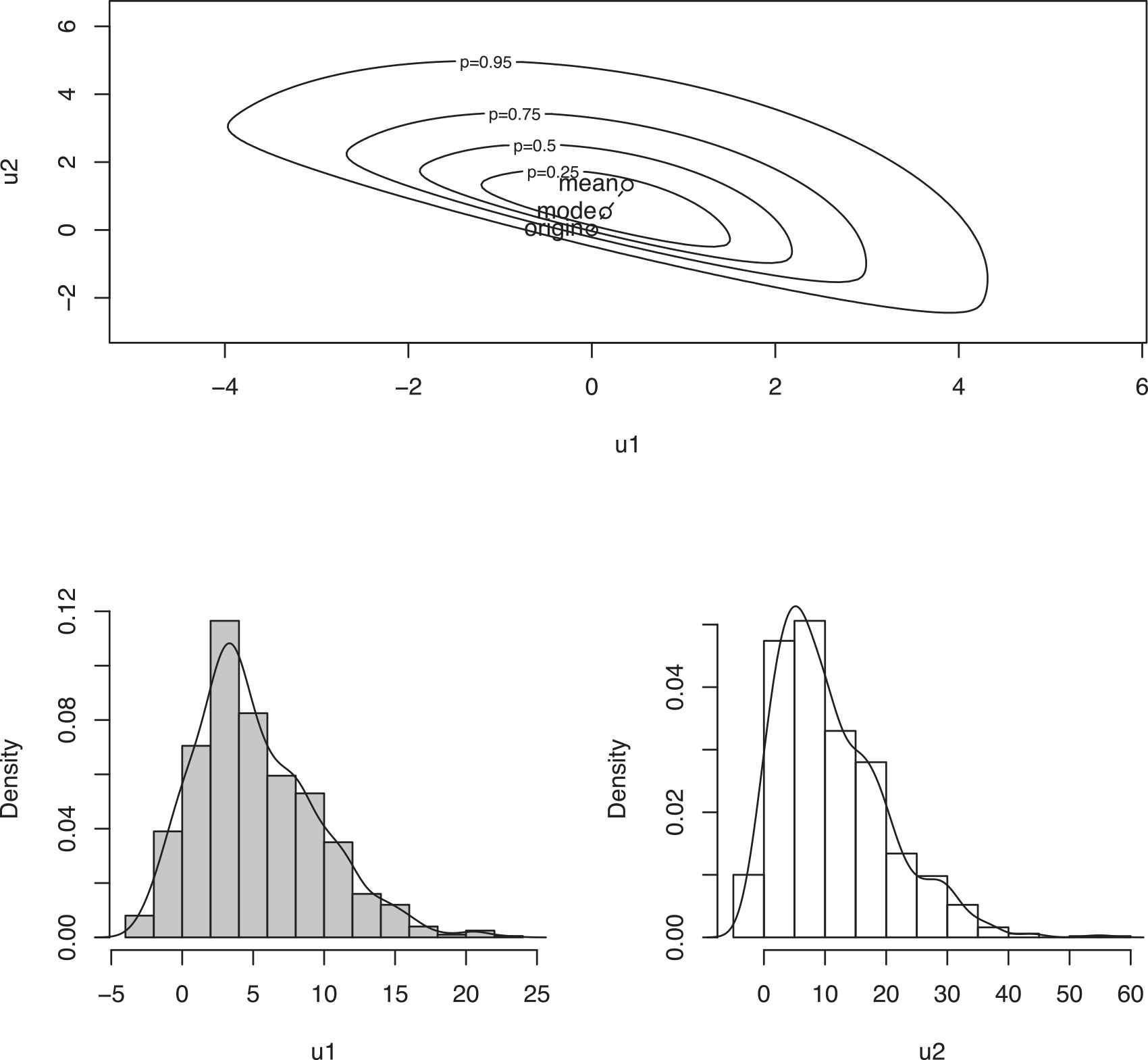
Contour plot of bivariate skew-normal density functions when
Now, suppose one is interested in the estimator of parameters in this model through the maximum likelihood approach. Then, corresponding logarithm of the likelihood function, say
By substituting this estimation into the expression in (3.5), one will obtain
We conduct some simulation studies using model (2.1) along with normal and skew-normal distributions in the following section. Moreover, we investigate the application of these methods in real-life data.
4. SIMULATION STUDIES AND APPLICATION
Here, we outline our simulation study to evaluate the performance of the parameters estimation for the SUR models given in Section 2. Suppose we have the following model:
To further identification of this model, we need to indicate a distribution for
We fix the parameter in our simulation studies as
To initiate our simulation studies, we take the sample size equal to
The results gained from our simulation studies for both the normal and skew-normal cases are given in Table 1. As seen, the table is partitioned into two parts. The three left- hand sides panels are related to the results coming from the normal assumption and the rest on the right belong to the skew-normal assumption both for error term. The distributions are indicated by N (Normal) and SN (Skew-Normal). Furthermore, the table includes estimate, standard deviation (SD), and effect size (ES).
| N-ML |
SN-ML |
|||||
|---|---|---|---|---|---|---|
| Parameter | Estimate | SD | ES | Estimate | SD | ES |
| 9.552 | 0.602 | 3.552 | 5.736 | 0.313 | 0.264 | |
| −3.001 | 0.018 | 0.001 | −3.003 | 0.011 | 0.003 | |
| −4.002 | 0.067 | 0.002 | −3.982 | 0.023 | 0.018 | |
| 18.11 | 0.751 | 9.11 | 8.711 | 0.451 | 0.289 | |
| 3.007 | 0.063 | 0.007 | 3.007 | 0.029 | 0.007 | |
| −2.013 | 0.068 | 0.013 | −1.969 | 0.037 | 0.031 | |
| 20.55 | 4.849 | 8.55 | 12.47 | 1.059 | 0.474 | |
| 41.42 | 5.543 | 30.42 | 11.25 | 3.377 | 0.258 | |
| −9.57 | 1.414 | 7.577 | −1.72 | 1.175 | 0.28 | |
| – | – | – | 2.210 | 0.691 | 0.210 | |
| – | – | – | 3.211 | 1.080 | 0.211 | |
The result of SUR model fitted according to the skew-normal and normal assumptions.
Based on the results in Table 1, the estimates for
One notes that the likelihood ratio test for the null hypothesis
| Criteria | N-ML | SN-ML |
|---|---|---|
| AIC | 13143.32 | 13035.198 |
| Log likelihood | −6560.66 | −6508.599 |
Criteria to compare two methods of model parameters estimate.
We were interested in applying the proposed model in this paper in real-life data. To do this, we used the Iranian rural households income and expenditure data collected in the year
A general description of the considered variables is provided in Table 3. Figures 2–4 present a geometric display of two important variables.
| Variable Names | Abbreviation Signs | Variable Type | Coding |
|---|---|---|---|
| Households expenditure | Quantitative | – | |
| Households income | Quantitative | – | |
| Family size | Quantitative | – | |
| Number of literate in household | Quantitative | – | |
| Number of employees in household | Quantitative | – | |
| Number of people with income | Quantitative | – | |
| Age | Quantitative | – | |
| Floor area | Quantitative | – | |
| Private car | Qualitative | 1: Use, 0: Nonuse | |
| Internet | Qualitative | 1: Use, 0: Nonuse | |
| Gas | Qualitative | 1: Use, 0: Nonuse | |
| Mobile | Qualitative | 1: Use, 0: Nonuse | |
| Agriculture self-employment income | Quantitative | – | |
| Nonagriculture self-employment income | Quantitative | – | |
| Miscellaneous income | Quantitative | – | |
| Non-monetary other incomes | Quantitative | – |
Description of variables utilized in model (4.4).
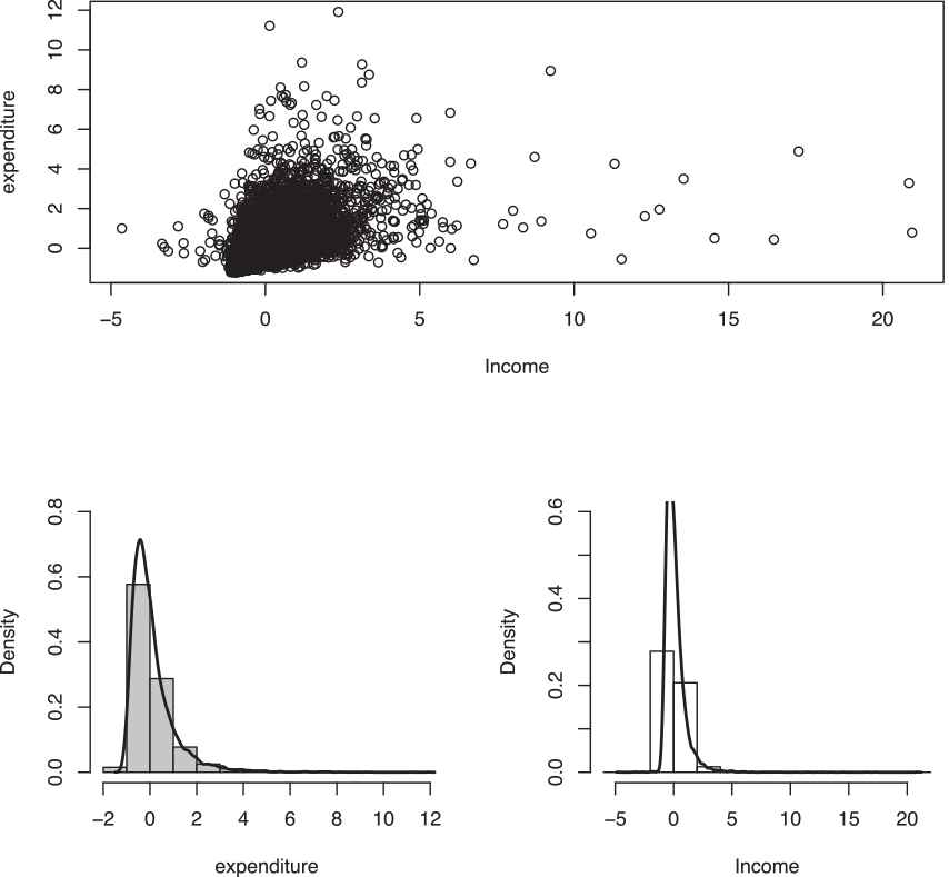
The scatter plot of Iranian rural households income and expenditure. Also the marginal histogram of each variable are provided in the lower panel.
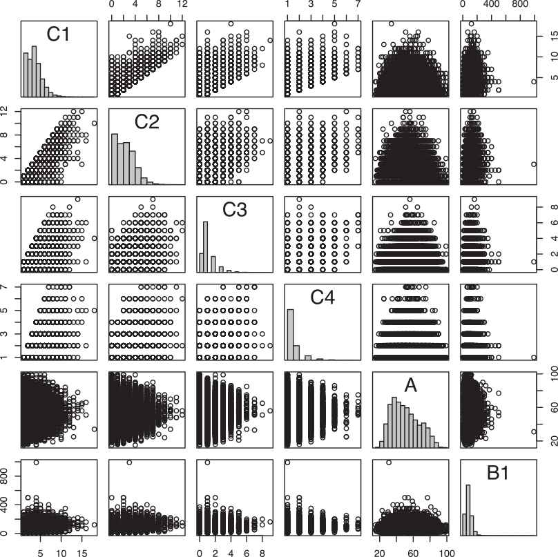
The pairs plot of quantitative variables described in Table 3.
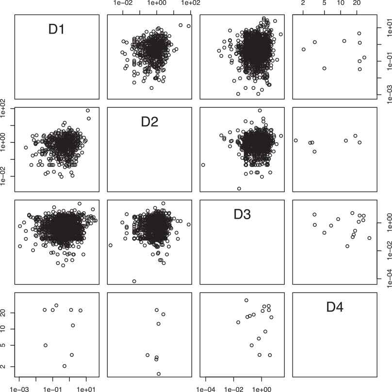
The pairs plot of quantitative variables described in Table 3.
To initiate the analysis, the validity of the normality assumption for the response variables should be tested. We used the Kolmogorov–Smirnov (KS) test statistics for this purpose. The results of the KS test was significant with p-value
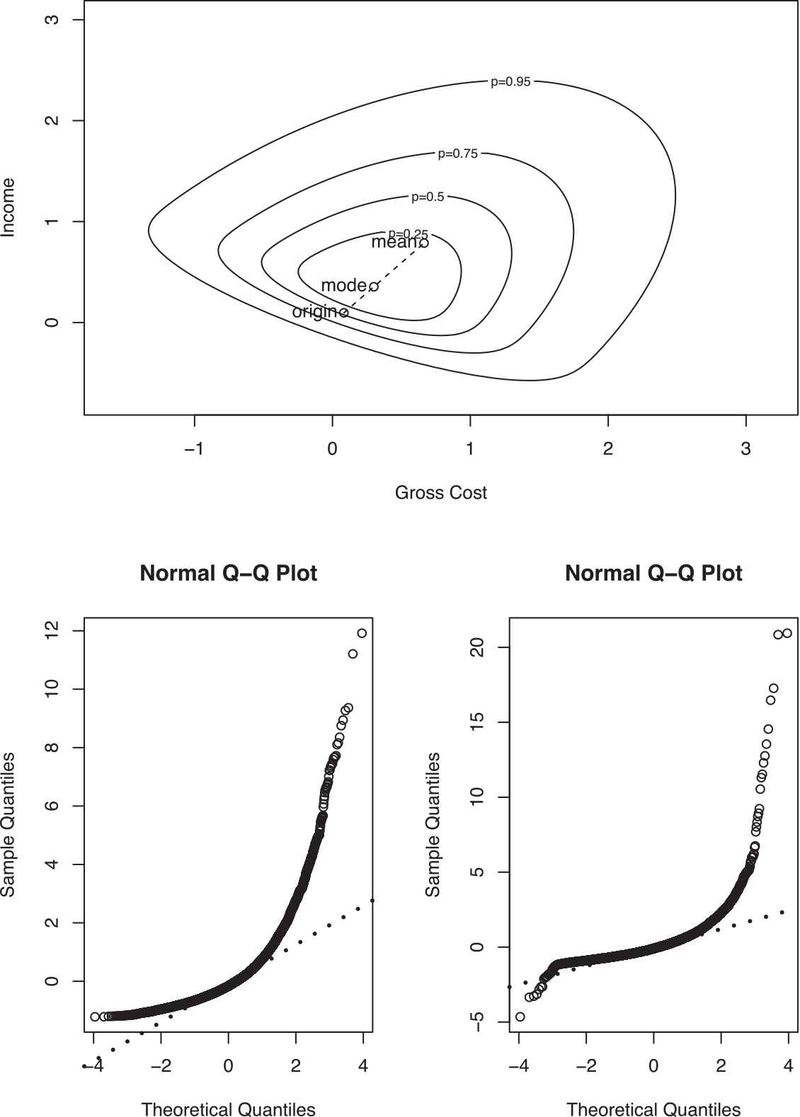
The contour plot of rural households income and expenditure along with the Q-Q plot for each variable.
The results from employing aforementioned models for our example are appeared in Table 4. As seen, it includes three panels. The first (second) panel shows the results for the first (second) equation of the model (4.4). Confining ourselves only to those significant estimates of the parameters at
| Estimation |
Sth.error |
|||
|---|---|---|---|---|
| Parameter | N-ML | SN-ML | N-ML | SN-ML |
| −1.50 | −1.34 | 0.047 | 0.006 | |
| 0.036 | 0.040 | 0.009 | 0.001 | |
| 0.082 | 0.046 | 0.010 | 0.002 | |
| 0.106 | 0.059 | 0.011 | 0.004 | |
| 0.061 | −0.024 | 0.014 | 0.004 | |
| 0.003 | 0.003 | 0.0006 | 0.0001 | |
| 0.004 | 0.002 | 0.0002 | 0.0005 | |
| 0.649 | 0.531 | 0.024 | 0.013 | |
| 0.689 | 0.490 | 0.051 | 0.032 | |
| 0.064 | 0.031 | 0.018 | 0.0085 | |
| 0.276 | 0.137 | 0.025 | 0.0064 | |
| 0 | −0.103 | 0.025 | 0.0038 | |
| 0.544 | 0.499 | 0.013 | 0.0039 | |
| 0.503 | 0.487 | 0.013 | 0.0039 | |
| 0.412 | 0.352 | 0.013 | 0.0039 | |
| 0.033 | 0.030 | 0.013 | 0.0038 | |
| 0.656 | 0.051 | 0.011 | 0.009 | |
| 0.084 | 0.009 | 0.009 | 0.001 | |
| 0.315 | 0.018 | 0.008 | 0.004 | |
| – | 1.181 | – | 0.104 | |
| – | 0.869 | – | 0.097 | |
The result of fitting the seemingly unrelated regression (SUR) model in (4.4) considering the skew-normal and normal distributions assumption for the response in the Iranian rural households income and expenditure data on year 2009.
Based on the results given in the first panel of Table 4, using facilities (including the Internet, gas, and mobile), has a direct effect on family households expenditure in Iran. In other words, using these facilities can increase family households expenditure. It is also seen that, family size, number of literate, employees, and people with income in household and age have direct link with family households expenditure. Moreover, regarding the second panel of Table 4, the agriculture self-employment, non-agriculture self-employment, miscellaneous income, and non-monetary other incomes have direct effect on the family incomes.
5. CONCLUSION
There are some examples of encountering with data having an asymmetric histogram. Considering some skew-normal distributions is usually a solution to construct a model. The problem will be harder if one should take SEMs into account. Confining to the SUR model, which is a particular case of SEM, we discussed the method of estimation for the parameters of this model in this paper. Here, the response variables were following the skew-normal distribution. Performance of the proposed method has been compared with an alternative case in which the normal density is incorrectly assumed for the error. Then, we applied the methods discussed in this paper on real data. Results shown superiority of our approach to other methods relied on normal distribution for the error. There is still room to extend the model in this paper. One of the possible options is to investigate the performance of the Bayesian approach on the SUR model with skew-normal assumption for the error term. Moreover, to check how other skew distributions such as skew-t density works on the SUR models worth to study.
CONFLICTS OF INTEREST
The author(s) declared no potential conflicts of interest with respect to the research, authorship, and/or publication of this article
Funding Statement
Receiving support from the Center of Excellence in Analysis of Spatio Temporal Correlated Data at Tarbiat Modares University.
APPENDIX
Theorem: For any fixed
In Equation (3.8),
Suppose
Hence,
As it can be seen, the first column and
As a general rule, the Hessian matrix is required if one is interested in utilizing the quasi-Newton algorithm. The relevant derivatives to construct such a matrix are as follows:
Notice that we used the property
On getting (5.7), we employed the following equality in which
The components of the second matrix in the last expression (5.7) are determined using (5.5). Assuming
If both
Footnotes
Two-stage Least Square
Three-stage Least Square
Generalized Method of Moments
Limited Information Maximum Likelihood
Fully Information Maximum Likelihood
REFERENCES
Cite this article
TY  - JOUR
AU  - Omid Akhgari
AU  - Mousa Golalizadeh
PY  - 2021
DA  - 2021/02/08
TI  - On Seemingly Unrelated Regression Model with Skew Error
JO  - Journal of Statistical Theory and Applications
SP  - 97
EP  - 110
VL  - 20
IS  - 1
SN  - 2214-1766
UR  - https://doi.org/10.2991/jsta.d.210126.002
DO  - 10.2991/jsta.d.210126.002
ID  - Akhgari2021
ER  -