
On Inference of Overlapping Coefficients in Two Inverse Lomax Populations
- DOI
- 10.2991/jsta.d.210107.002How to use a DOI?
- Keywords
- β-Divergence; Kernel density Estimation; Bandwidth
- Abstract
Overlapping coefficient is a direct measure of similarity between two distributions which is recently becoming very useful. This paper investigates estimation for some well-known measures of overlap, namely Matusita's measure
- Copyright
- © 2021 The Authors. Published by Atlantis Press B.V.
- Open Access
- This is an open access article distributed under the CC BY-NC 4.0 license (http://creativecommons.org/licenses/by-nc/4.0/).
1. INTRODUCTION
Inverse Lomax distribution is a special case of the generalized beta distribution of the second kind. It is one of the notable lifetime models in statistical applications. The inverse Lomax distribution is one of significant lifetime models. Kleiber and Kotz [1] used this inverse Lomax distribution to get Lorenz ordering relationship among ordered statistics. McKenzie et al. [2] applied this life time distribution on geophysical data on the sizes of land fires in the California State, United States.
The overlapping coefficients (
Matusia's measure [3]
Weitzman's measure [4]
OVL-based Kullback and Leibler [5]
with
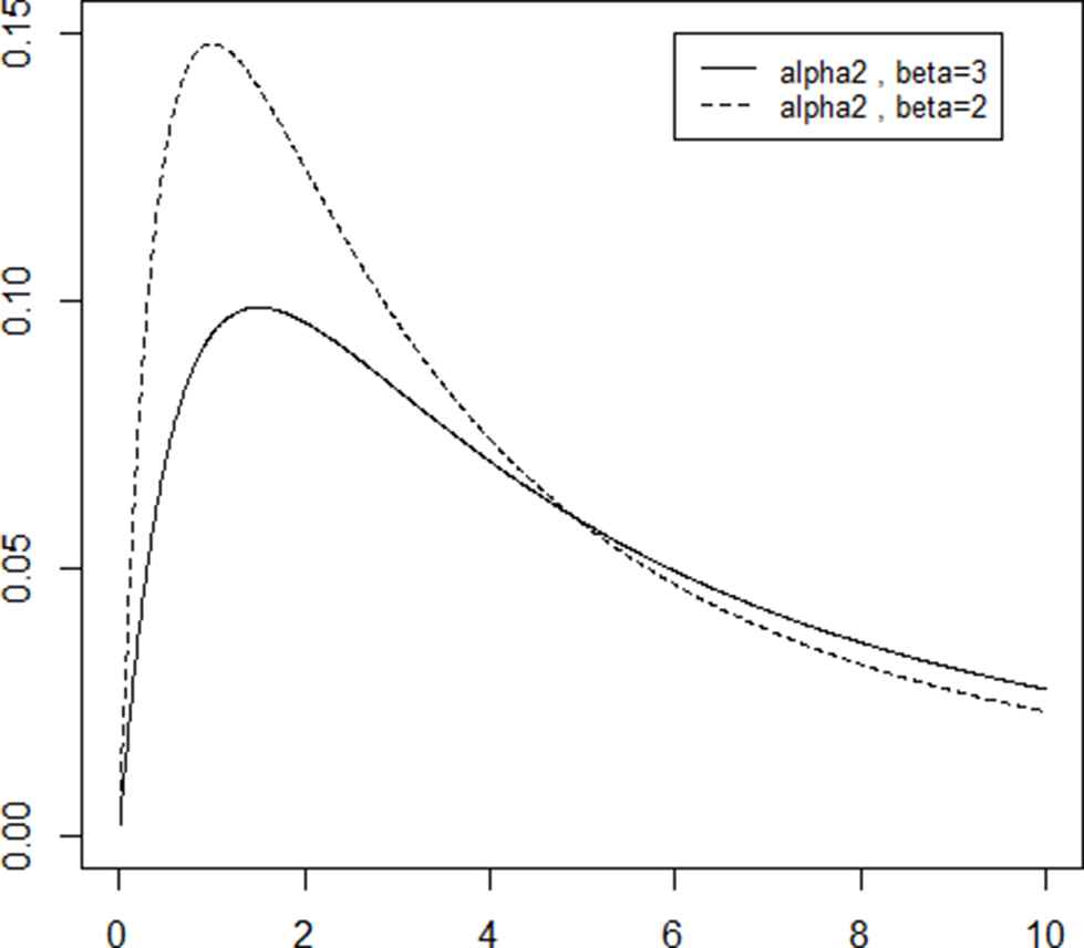
The overlap of two inverse Lomax densities.
The mathematical structure of these measures is complicated; there are no results available on the exact sampling distributions of the commonly used OVL estimators. Researchers such as Smith [6] derived formulas for estimating the mean and the variance of discrete version of Weitzman's measure using the delta method. Mishra et al. [7] gave small and large sample properties of the sampling distribution for a function of
In this article, we consider the point and interval estimation for some measures of overlap (OVL) for two inverse Lomax populations with different shape parameters using “Simple Random Sample (SRS) and Ranked Set Sampling (RSS) and Bayesian methodology.”
The first method (RSS, McIntyre [15]) was earlier applied by Helu and Samawi [16] for the point and interval estimation of the overlapping coefficients for two Lomax distributions. We will use their methodology for the point estimate and interval in the case of inverse Lomax distribution. The second approach, we use another method for parameter estimation using Bayesian inference [17].
The primary purpose of this study is to compare the confidence intervals for the overlap coefficients (
2. OVL MEASURES FOR INVERSE LOMAX DISTRIBUTION
A random variable
Consider the random variable
We consider another variable with
The computation or estimation of OVL for two inverse Lomax distributions, with density functions:
Let
Figure 2 shows curves of the three overlap measures according to R All three measures are monotone for all R > 0.
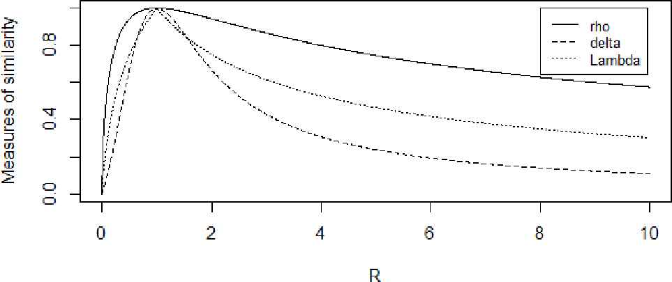
Measures of similarity as functions of R.
Proposition 2.1.
For OVLs defined earlier,
Proposition 2.2.
All four OVLs possess properties of reciprocity, invariance and piecewise monotonicity
3. STATISTICAL INFERENCE USING SRS
3.1. Estimation
As in Helu and Samawi [16], parallel results to those of the two Lomax populations can be established for the inverse Lomax populations.
Suppose
The maximum likelihood estimators (MLEs) based on the two samples are given by
From the first sample:
From the second sample:
The maximum likelihood estimators
Consequently, the means and variances of those
Then we may define an estimate of
Therefore, using the relationship between gamma distribution and chi-square distribution and the fact that the two samples are independent, it is easy to show that
Also, an unibiased estimate
Clearly,
Since the
3.2. Asymptotic Properties
Let
Theorem 3.1.
Let
Proof.
Let function
Then the variance of
Since, in this case,
Similar arguments can be used for the other overlaps coefficients.
Theorem 3.2.
Using Taylor series expansion, then for
Proof.
Again by using the well-known Delta method (Taylor series expansion) the asymptotic bias of the OVL measures can be obtained as follows:
Since, in this case,
3.3. Interval Estimation
For large sample, normal approximation to the sampling distribution, using the delta method, works fairly well. Therefore, the asymptotic
These confidence intervals are not the best because of the bias involved in
4. STATISTICAL INFERENCE USING RSS
4.1. Estimation
Similar to the previous section, suppose
From the first sample:
From the second sample:
Note that, it is easy to show that
Also,
Thus, we have
4.2. Asymptotic Properties
Let
Corollary 4.1.
Let
Proof.
Same proof of Theorem 3.1, replacing
Corollary 4.2.
Using Taylor series expansion, then for
Proof.
Same proof of Theorem 3.2, replacing
4.3. Interval Estimation
Similar to the case of SRS and RSS, the asymptotic
These confidence intervals are not the best because of the bias involved in
5. STATISTICAL INFERENCE USING BAYESIAN APPROACH
In recent decades, the Bayes viewpoint, as a powerful and valid alternative to traditional statistical perspectives, has received frequent attention for statistical inference. In our study normal approximations for the shape parameter
5.1. Estimation
Jeffery's Prior: Using Jeffery's prior for the scale parameter
Using (20) and (13) we get the posterior distribution for
The log posterior is
The first derivative is
and the posterior mode is obtained asFrom the first sample:
From the second sample:
Using simple transformation, it can be shown that
A consequent estimate of
Also, an unibiased estimate
Thus, we have
The asymptotic variance of the
With the asymptotic bias given by
5.2. Interval Estimation
The
Using these estimates the bias corrected interval, the
6. SIMULATION
In our simulation study we include the following:
The performance of the
Where
Tables 1 and 2 show the asymptotic relative efficiencies for the OVL measures using RSS relative to using SRS.
| R | 2 | 3 | 4 | 5 | 2 | 3 | 4 | 5 | 2 | 3 | 4 | 5 | |||
|---|---|---|---|---|---|---|---|---|---|---|---|---|---|---|---|
| 0.10 | 2 | 0.9830 | 0.9795 | 0.9790 | 0.9791 | 0.990 | 0.9882 | 0.9879 | 0.9879 | 0.9998 | 0.9999 | 0.9998 | 0.9998 | ||
| 3 | 0.9864 | 0.9839 | 0.9837 | 0.9840 | 0.9921 | 0.9908 | 0.9907 | 0.9908 | 0.9999 | 0.9999 | 0.9998 | 0.9999 | |||
| 4 | 0.9882 | 0.9861 | 0.9861 | 0.9865 | 0.9932 | 0.9921 | 0.9921 | 0.9923 | 0.9999 | 0.9999 | 0.9999 | 0.9999 | |||
| 5 | 0.9865 | 0.9874 | 0.9876 | 0.9880 | 0.9923 | 0.9928 | 0.9929 | 0.9932 | 0.9999 | 0.9999 | 0.9999 | 0.9999 | |||
| 0.5 | 2 | 0.9021 | 0.9012 | 0.8958 | 0.8940 | 0.9814 | 0.9779 | 0.9772 | 0.9772 | 0.9828 | 0.9796 | 0.9791 | 0.9791 | ||
| 3 | 0.9331 | 0.9164 | 0.9129 | 0.9125 | 0.9852 | 0.9825 | 0.9823 | 0.9825 | 0.9864 | 0.9839 | 0.9838 | 0.9840 | |||
| 4 | 0.9401 | 0.9252 | 0.9228 | 0.9232 | 0.9872 | 0.9848 | 0.9849 | 0.9853 | 0.9882 | 0.9861 | 0.9862 | 0.9865 | |||
| 5 | 0.9446 | 0.9308 | 0.9292 | 0.9302 | 0.9884 | 0.9863 | 0.9865 | 0.9870 | 0.9893 | 0.9875 | 0.9876 | 0.9881 | |||
| 0.8 | 2 | 0.8510 | 0.8036 | 0.7854 | 0.7764 | 0.8848 | 0.8523 | 0.8415 | 0.8369 | 0.8861 | 0.8541 | 0.8435 | 0.8391 | ||
| 3 | 0.8647 | 0.8177 | 0.8001 | 0.7929 | 0.8991 | 0.8693 | 0.8607 | 0.8579 | 0.9004 | 0.8712 | 0.8628 | 0.8601 | |||
| 4 | 0.8732 | 0.8270 | 0.8112 | 0.8045 | 0.9077 | 0.8797 | 0.8727 | 0.8711 | 0.9090 | 0.8816 | 0.8749 | 0.8733 | |||
| 5 | 0.8791 | 0.8340 | 0.8188 | 0.8129 | 0.9133 | 0.8868 | 0.8809 | 0.8802 | 0.9146 | 0.8886 | 0.8829 | 0.8823 | |||
Asymptotic relative efficiency of OVL estimates using RSS relative to using SRS,
| R | 2 | 3 | 4 | 5 | 2 | 3 | 4 | 5 | 2 | 3 | 4 | 5 | |||
|---|---|---|---|---|---|---|---|---|---|---|---|---|---|---|---|
| 0.10 | 2 | 0.9931 | 0.9940 | 0.9945 | 0.9948 | 0.9961 | 0.9966 | 0.9997 | 0.9971 | 0.9999 | 0.9999 | 0.9999 | 0.9999 | ||
| 3 | 0.9943 | 0.9952 | 0.9957 | 0.9960 | 0.9968 | 0.9973 | 0.9976 | 0.9978 | 0.9999 | 0.9999 | 0.9999 | 0.9999 | |||
| 4 | 0.9949 | 0.9958 | 0.9963 | 0.9952 | 0.9971 | 0.9977 | 0.9979 | 0.9981 | 0.9999 | 0.9999 | 0.9999 | 0.9999 | |||
| 5 | 0.9952 | 0.9962 | 0.9967 | 0.9970 | 0.9973 | 0.9979 | 0.9982 | 0.9983 | 0.9999 | 0.9999 | 0.9999 | 0.9999 | |||
| 0.5 | 2 | 0.9552 | 0.9603 | 0.9631 | 0.9650 | 0.9925 | 0.9935 | 0.9940 | 0.9943 | 0.9931 | 0.9940 | 0.9945 | 0.9948 | ||
| 3 | 0.9621 | 0.9677 | 0.9707 | 0.9727 | 0.9937 | 0.9948 | 0.9953 | 0.9957 | 0.9943 | 0.9952 | 0.9957 | 0.9961 | |||
| 4 | 0.9655 | 0.9713 | 0.9746 | 0.9767 | 0.9944 | 0.9954 | 0.9960 | 0.9964 | 0.9949 | 0.9958 | 0.9963 | 0.9967 | |||
| 5 | 0.9677 | 0.9736 | 0.9770 | 0.9791 | 0.9948 | 0.9958 | 0.9964 | 0.9967 | 0.9952 | 0.9962 | 0.9967 | 0.9970 | |||
| 0.8 | 2 | 0.8430 | 0.8516 | 0.8575 | 0.8616 | 0.9146 | 0.9225 | 0.9272 | 0.9304 | 0.9165 | 0.9243 | 0.9290 | 0.9321 | ||
| 3 | 0.8578 | 0.8694 | 0.8772 | 0.8828 | 0.9259 | 0.9351 | 0.9406 | 0.9442 | 0.9276 | 0.9370 | 0.9421 | 0.9456 | |||
| 4 | 0.8663 | 0.8798 | 0.8889 | 0.8953 | 0.9319 | 0.9419 | 0.9477 | 0.9517 | 0.9335 | 0.9433 | 0.9491 | 0.9530 | |||
| 5 | 0.8718 | 0.8866 | 0.8966 | 0.9036 | 0.9357 | 0.9461 | 0.9523 | 0.9564 | 0.9373 | 0.9475 | 0.9536 | 0.9576 | |||
Asymptotic relative efficiency of OVL estimates using RSS relative to using SRS,
Tables 1 and 2 shows that, using
Tables 3 and 4 indicate that the bias of the proposed OVL estimators is negligible in most cases and
| SRS |
RSS |
BAYES |
|||||||||||||||||||||||||
|---|---|---|---|---|---|---|---|---|---|---|---|---|---|---|---|---|---|---|---|---|---|---|---|---|---|---|---|
| (2,2) | 0.026 | 0.283 | 0.288 | 0.002 | 0.215 | 0.024 | 0.001 | 0.024 | 0.146 | 0.035 | 0.437 | 0.237 | 0.002 | 0.340 | 0.020 | 0.001 | 0.040 | 0.120 | 0.163 | 0.881 | 0.288 | 0.324 | 0.999 | 0.024 | 0.002 | 0.018 | 0.393 |
| (2,3) | 0.021 | 0.250 | 0.261 | 0.013 | 0.193 | 0.022 | 0.0009 | 0.022 | 0.131 | 0.027 | 0.392 | 0.208 | 0.002 | 0.303 | 0.017 | 0.001 | 0.035 | 0.106 | 0.055 | 0.736 | 0.168 | 0.110 | 0.999 | 0.014 | 0.0007 | 0.009 | 0.256 |
| (3,3) | 0.017 | 0.0.230 | 0.231 | 0.001 | 0.173 | 0.019 | 0.0007 | 0.0196 | 0.131 | 0.019 | 0.337 | 0.175 | 0.001 | 0.258 | 0.015 | 0.001 | 0.029 | 0.089 | 0.105 | 0.831 | 0.231 | 0.208 | 0.999 | 0.019 | 0.001 | 0.012 | 0.393 |
| (3,4) | 0.014 | 0.214 | 0.214 | 0.001 | 0.161 | 0.018 | 0.0006 | 0.018 | 0.109 | 0.017 | 0.317 | 0.163 | 0.001 | 0.242 | 0.014 | 0.001 | 0.028 | 0.083 | 0.060 | 0.717 | 0.159 | 0.098 | 0.999 | 0.103 | 0.0006 | 0.007 | 0.292 |
| (4,4) | 0.012 | 0.199 | 0.198 | 0.0008 | 0.150 | 0.0170 | 0.0005 | 0.017 | 0.100 | 0.014 | 0.296 | 0.151 | 0.0009 | 0.225 | 0.013 | 0.0006 | 0.026 | 0.077 | 0.077 | 0.789 | 0.198 | 0.153 | 0.999 | 0.0167 | 0.001 | 0.009 | 0.393 |
| (5,5) | 0.010 | 0.178 | 0.176 | 0.0006 | 0.133 | 0.015 | 0.0004 | 0.015 | 0.090 | 0.011 | 0.267 | 0.135 | 0.0007 | 0.202 | 0.011 | 0.0005 | 0.023 | 0.069 | 0.061 | 0.752 | 0.176 | 0.122 | 0.999 | 0.015 | 0.015 | 0.068 | 0.393 |
| (2,2) | 0.047 | 0.627 | 0.192 | 0.020 | 0.295 | 0.212 | 0.073 | 0.282 | 0.816 | 0.064 | 0.799 | 0.158 | 0.027 | 0.453 | 0.174 | 0.099 | 0.436 | 0.671 | 0.1333 | 0.9158 | 0.1923 | 0.1590 | 0.9268 | 0.2121 | 0.1461 | 0.2140 | 2.1931 |
| (2,3) | 0.038 | 0.585 | 0.172 | 0.159 | 0.266 | 0.190 | 0.058 | 0.255 | 0.730 | 0.049 | 0.759 | 0.139 | 0.021 | O.407 | 0.153 | 0.076 | 0.391 | 0.589 | 0.0454 | 0.7993 | 0.1122 | 0.0541 | 08213 | 0.1237 | 0.0497 | 0.1137 | 1.4303 |
| (3,3) | 0.030 | 0.543 | 0.154 | 0.013 | 0.240 | 0.170 | 0.047 | 0.230 | 0.654 | 0.035 | 0.699 | 0.117 | 0.015 | 0.350 | 0.129 | 0.054 | 0.336 | 0.495 | 0.0857 | 0.8773 | 0.1542 | 0.1022 | 0.8925 | 0.1701 | 0.0931 | 0.1396 | 2.1931 |
| (3,4) | 0.026 | 0.514 | 0.143 | 0.011 | 0.223 | 0.157 | 0.040 | 0.214 | 0.606 | 0.030 | 0.675 | 0.109 | 0.013 | 0.330 | 0.120 | 0.047 | 0.317 | 0.463 | 0.0405 | 0.7825 | 0.1060 | 0.0483 | 0.8056 | 0.1169 | 0.0044 | 0.0893 | 1.6271 |
| (4,4) | 0.022 | 0.485 | 0.132 | 0.009 | 0.208 | 0.146 | 0.035 | 0.199 | 0.562 | 0.026 | 0.646 | 0.101 | 0.011 | 0.308 | 0.111 | 0.0403 | 0.296 | 0.429 | 0.0631 | 0.8434 | 0.1324 | 0.0751 | 0.8617 | 0.1460 | 0.0693 | 0.1033 | 2.1931 |
| (5,5) | 0.018 | 0.443 | 0.118 | 0.007 | 0.186 | 0.130 | 0.027 | 0.178 | 0.500 | 0.021 | 0.604 | 0.090 | 0.009 | 0.278 | 0.099 | 0.032 | 0.267 | 0.383 | 0.0500 | 0.8132 | 0.1178 | 0.0597 | 0.8340 | 0.1299 | 0.0549 | 0.0820 | 2.1931 |
| (2,2) | 0.043 | 0.851 | 0.086 | 0.091 | 0.669 | 0.334 | 0.167 | 0.670 | 0.608 | 0.058 | 0.936 | 0.071 | 0.126 | 0.829 | 0.275 | 0.226 | 0.829 | 0.501 | 0.0984 | 0.9661 | 0.0865 | 0.3253 | 0.9545 | 0.3341 | 0.3334 | 0.5572 | 1.6351 |
| (2,3) | 0.034 | 0.823 | 0.077 | 0.073 | 0.627 | 0.299 | 0.133 | 0.628 | 0.544 | 0.044 | 0.920 | 0.062 | 0.096 | 0.793 | 0.242 | 0.174 | 0.793 | 0.439 | 0.0335 | 0.9092 | 0.0504 | 0.1107 | 0.8817 | 0.1950 | 0.1135 | 0.3306 | 1.0664 |
| (3,3) | 0.027 | 0.793 | 0.069 | 0.059 | 0.585 | 0.268 | 0.107 | 0.586 | 0.488 | 0.031 | 0.891 | 0.052 | 0.067 | 0.738 | 0.203 | 0.123 | 0.738 | 0.369 | 0.0633 | 0.9487 | 0.0693 | 0.2093 | 0.9319 | 0.2680 | 0.2145 | 0.3962 | 1.6351 |
| (3,4) | 0.023 | 0.769 | 0.064 | 0.050 | 0.556 | 0.248 | 0.092 | 0.557 | 0.452 | 0.027 | 0.878 | 0.049 | 0.059 | 0.715 | 0.189 | 0.107 | 0.715 | 0.345 | 0.0299 | 0.8999 | 0.0476 | 0.0988 | 0.8701 | 0.1842 | 0.1013 | 0.2649 | 1.2131 |
| (4,4) | 0.020 | 0.745 | 0.060 | 0.043 | 0.527 | 0.230 | 0.079 | 0.527 | 0.419 | 0.023 | 0.862 | 0.045 | 0.0500 | 0.687 | 0.175 | 0.092 | 0.688 | 0.319 | 0.0467 | 0.9323 | 0.0596 | 0.1543 | 0.9107 | 0.2301 | 0.1581 | 0.3031 | 1.6351 |
| (5,5) | 0.016 | 0.705 | 0.053 | 0.034 | 0.483 | 0.204 | 0.063 | 0.484 | 0.373 | 0.019 | 0.836 | 0.041 | 0.040 | 0.646 | 0.157 | 0.074 | 0.646 | 0.286 | 0.03697 | 0.9169 | 0.0530 | 0.1222 | 0.8910 | 0.2048 | 0.1252 | 0.2443 | 1.6351 |
| (2,2) | 0.038 | 0.968 | 0.032 | 0.344 | 0.942 | 0.405 | 0.201 | 0.934 | 0.253 | 0.051 | 0.988 | 0.026 | 0.466 | 0.977 | 0.333 | 0.272 | 0.974 | 0.208 | 0.0801 | 0.9926 | 0.0322 | 0.8483 | 0.0.9897 | 0.4046 | 0.4022 | 0.8896 | 0.6793 |
| (2,3) | 0.030 | 0.961 | 0.029 | 0.275 | 0.928 | 0.362 | 0.161 | 0.920 | 0.226 | 0.040 | 0.984 | 0.023 | 0.359 | 0.971 | 0.292 | 0.210 | 0.987 | 0.183 | 0.0273 | 0.9788 | 0.0187 | 0.2892 | 0.9705 | 0.2361 | 0.1369 | 0.7130 | 0.4430 |
| (3,3) | 0.024 | 0.952 | 0.026 | 0.221 | 0.913 | 0.324 | 0.129 | 0.952 | 0.203 | 0.028 | 0.978 | 0.019 | 0.253 | 0.959 | 0.245 | 0.148 | 0.954 | 0.153 | 0.0515 | 0.9886 | 0.0258 | 0.5463 | 0.9841 | 0.3245 | 0.2587 | 0.7815 | 0.6793 |
| (3,4) | 0.021 | 0.945 | 0.024 | 0.200 | 0.901 | 0.301 | 0.111 | 0.889 | 0.188 | 0.024 | 0.975 | 0.018 | 0.221 | 0.954 | 0.230 | 0.129 | 0.948 | 0.143 | 0.0243 | 0.9763 | 0.0177 | 0.2580 | 0.9672 | 0.2230 | 0.1222 | 0.6235 | 0.5040 |
| (4,4) | 0.018 | 0.937 | 0.022 | 0.163 | 0.887 | 0.279 | 0.095 | 0.874 | 0.174 | 0.021 | 0.971 | 0.017 | 0.199 | 0.947 | 0.212 | 0.111 | 0.939 | 0.133 | 0.0379 | 0.9846 | 0.0221 | 0.4027 | 0.9786 | 0.2786 | 0.1907 | 0.6784 | 0.6793 |
| (5,5) | 0.014 | 0.922 | 0.020 | 0.129 | 0.864 | 0,248 | 0.075 | 0.849 | 0.155 | 0.017 | 0.964 | 0.015 | 0.152 | 0.935 | 0.190 | 0.089 | 0.926 | 0.119 | 0.0300 | 0.9807 | 0.0197 | 0.3189 | 0.9732 | 0.2479 | 0.1510 | 0.5904 | 0.6793 |
Bias, ratio, and length of interval (L.), using RSS, SRS and Baye,
| SRS |
RSS |
BAYES |
|||||||||||||||||||||||||
|---|---|---|---|---|---|---|---|---|---|---|---|---|---|---|---|---|---|---|---|---|---|---|---|---|---|---|---|
| (2,2) | 0.005 | 0.125 | 0.123 | 0.0003 | 0.094 | 0.0104 | 0.0002 | 0.0105 | 0.0628 | 0.0057 | 0.1923 | 0.0956 | 0.0003 | 0.1445 | 0.0080 | 0.0002 | 0.0162 | 0.0486 | 0.0300 | 0.1235 | 0.1235 | 0.0596 | 0.9985 | 0.0104 | 0.0004 | 0.003 | 0.393 |
| (2,3) | 0.004 | 0.114 | 0.112 | 0.0002 | 0.085 | 0.009 | 0.0002 | 0.009 | 0.0571 | 0.0047 | 0.1761 | 0.0873 | 0.0003 | 0.1321 | 0.0073 | 0.0002 | 0.0148 | 0.0444 | 0.0109 | 0.4352 | 0.0746 | 0.0217 | 0.9962 | 0.0063 | 0.0001 | 0.002 | 0.261 |
| (3,3) | 0.003 | 0.102 | 0.1005 | 0.0002 | 0.0765 | 0.008 | 0.0001 | 0.0085 | 0.051 | 0.0038 | 0.1580 | 0.0781 | 0.0002 | 0.1183 | 0.0065 | 0.0002 | 0.0132 | 0.0397 | 0.0199 | 0.5459 | 0.1005 | 0.0395 | 0.9979 | 0.0084 | 0.0003 | 0.002 | 0.393 |
| (3,4) | 0.003 | 0.0957 | 0.0939 | 0.0017 | 0.0714 | 0.0079 | 0.0001 | 0.0079 | 0.0477 | 0.0033 | 0.1481 | 0.0730 | 0.0002 | 0.1108 | 0.0061 | 0.0001 | 0.0124 | 0.0371 | 0.0097 | 0.4143 | 0.0702 | 0.01929 | 0.9957 | 0.0059 | 0.0002 | 0.001 | 0.294 |
| (4,4) | 0.002 | 0.0887 | 0.0869 | 0.0001 | 0.0662 | 0.007 | 0.000 | 0.0073 | 0.0442 | 0.0028 | 0.1373 | 0.0676 | 0.0002 | 0.1027 | 0.0057 | 0.0001 | 0.0114 | 0.0344 | 0.0149 | 0.4908 | 0.0073 | 0.0295 | 0.9971 | 0.0073 | 0.0002 | 0.001 | 0.393 |
| (5,5) | 0.002 | 0.0793 | 0.0777 | 0.0001 | 0.0592 | 0.0065 | 0.000 | 0.0066 | 0.0395 | 0.0023 | 0.1230 | 0.0605 | 0.0001 | 0.0920 | 0.0059 | 0.0000 | 0.0102 | 0.0307 | 0.0119 | 0.4496 | 0.0777 | 0.0236 | 0.9965 | 0.0065 | 0.0001 | 0.001 | 0.393 |
| (2,2) | 0.009 | 0.327 | 0.0825 | 0.0036 | 0.1312 | 0.0910 | 0.013 | 0.1254 | 0.3501 | 0.0104 | 0.4721 | 0.0639 | 0.004 | 0.2007 | 0.0704 | 0.0161 | 0.1921 | 0.2711 | 0.024 | 0.6993 | 0.0825 | 0.0293 | 0.7269 | 0.0910 | 0.027 | 0.040 | 2.193 |
| (2,3) | 0.007 | 0.300 | 0.0750 | 0.003 | 0.1194 | 0.0830 | 0.011 | 0.114 | 0.3184 | 0.0087 | 0.439 | 0.0583 | 0.004 | 0.1839 | 0.0643 | 0.0134 | 0.1759 | 0.2475 | 0.009 | 0.5086 | 0.0498 | 0.0107 | 0.5386 | 0.0549 | 0.009 | 0.022 | 1.456 |
| (3,3) | 0.006 | 0.2709 | 0.0671 | 0.024 | 0.1071 | 0.0741 | 0.009 | 0.1023 | 0.2849 | 0.0069 | 0.4007 | 0.0522 | 0.003 | 0.1650 | 0.0575 | 0.0107 | 0.1578 | 0.2213 | 0.016 | 0.6229 | 0.0671 | 0.0194 | 0.6527 | 0.0741 | 0.018 | 0.027 | 2.193 |
| (3,4) | 0.005 | 0.2542 | 0.0627 | 0.0021 | 0.1000 | 0.0691 | 0.008 | 0.0956 | 0.2660 | 0.0061 | 0.3786 | 0.0488 | 0.002 | 0.1546 | 0.0538 | 0.0094 | 0.1478 | 0.2070 | 0.008 | 0.4861 | 0.0469 | 0.0094 | 0.5157 | 0.517 | 0.009 | 0.017 | 1.641 |
| (4,4) | 0.004 | 0.2365 | 0.0580 | 0.0018 | 0.0927 | 0.0640 | 0.007 | 0.0885 | 0.2463 | 0.0052 | 0.3541 | 0.0452 | 0.002 | 0.1434 | 0.050 | 0.0081 | 0.1371 | 0.1917 | 0.012 | 0.5670 | 0.0581 | 0.0145 | 0.5974 | 0.0640 | 0.013 | 0.020 | 2.103 |
| (5,5) | 0.003 | 0.2125 | 0.0519 | 0.0014 | 0.0823 | 0.0572 | 0.005 | 0.079 | 0.2201 | 0.0042 | 0.3208 | 0.0404 | 0.002 | 0.1285 | 0.0446 | 0.0064 | 0.1228 | 0.1714 | 0.009 | 0.5239 | 0.0520 | 0.0116 | 0.5541 | 0.0572 | 0.011 | 0.016 | 2.193 |
| (2,2) | 0.008 | 0.5710 | 0.0371 | 0.0168 | 0.3605 | 0.1434 | 0.031 | 0.3609 | 0.2610 | 0.0094 | 0.7328 | 0.0287 | 0.020 | 0.5136 | 0.1110 | 0.0368 | 0.5140 | 0.2021 | 0.018 | 0.8489 | 0.0371 | 0.0599 | 0.8086 | 0.1434 | 0.061 | 0.123 | 1.635 |
| (2,3) | 0.006 | 0.5346 | 0.0338 | 0.0139 | 0.3316 | 0.1304 | 0.025 | 0.3319 | 0.2374 | 0.0078 | 0.7011 | 0.0262 | 0.017 | 0.4795 | 0.1014 | 0.0307 | 0.4799 | 0.1845 | 0.007 | 0.6962 | 0.0224 | 0.0218 | 0.6386 | 0.0866 | 0.022 | 0.068 | 1.085 |
| (3,3) | 0.005 | 0.4926 | 0.0302 | 0.011 | 0.3001 | 0.1167 | 0.0203 | 0.3003 | 0.2124 | 0.0062 | 0.6604 | 0.0235 | 0.0134 | 0.4391 | 0.0907 | 0.0245 | 0.4395 | 0.1650 | 0.0120 | 0.7942 | 0.0302 | 0.0397 | 0.7455 | 0.1167 | 0.0407 | 0.081 | 1.635 |
| (3,4) | 0.004 | 0.4673 | 0.0282 | 0.0097 | 0.2818 | 0.1089 | 0.0177 | 0.2821 | 0.1983 | 0.0055 | 0.6353 | 0.0219 | 0.0117 | 0.4158 | 0.0848 | 0.0215 | 0.4162 | 0.1543 | 0.0059 | 0.6745 | 0.0211 | 0.0194 | 0.6158 | 0.0815 | 0.0199 | 0.053 | 1.221 |
| (4,4) | 0.004 | 0.4396 | 0.0261 | 0.0083 | 0.2624 | 0.1009 | 0.0152 | 0.2627 | 0.1837 | 0.0047 | 0.6059 | 0.0203 | 0.0101 | 0.389 | 0.0785 | 0.0184 | 0.3901 | 0.1429 | 0.0089 | 0.7489 | 0.0261 | 0.0297 | 0.6952 | 0.1001 | 0.004 | 0.061 | 1.635 |
| (5,5) | 0.004 | 0.4396 | 0.0261 | 0.0083 | 0.2624 | 0.1010 | 0.0152 | 0.2627 | 0.1837 | 0.0038 | 0.5630 | 0.0182 | 0.0081 | 0.3540 | 0.0702 | 0.0147 | 0.3544 | 0.1278 | 0.0072 | 0.7106 | 0.0233 | 0.0236 | 0.6538 | 0.0902 | 0.0243 | 0.0488 | 1.635 |
| (2,2) | 0.007 | 0.8576 | 0.0137 | 0.0633 | 0.7682 | 0.1736 | 0.037 | 0.7469 | 0.1084 | 0.0084 | 0.9325 | 0.0107 | 0.0759 | 0.8806 | 0.1344 | 0.0444 | 0.8669 | 0.0840 | 0.0300 | 0.6249 | 0.1235 | 0.0596 | 0.9986 | 0.0104 | 0.0004 | 0.003 | 0.393 |
| (2,3) | 0.006 | 0.8348 | 0.0125 | 0.0524 | 0.7373 | 0.1579 | 0.0306 | 0.7146 | 0.0986 | 0.0070 | 0.9205 | 0.0097 | 0.0633 | 0.8615 | 0.1227 | 0.03670 | 0.8461 | 0.0766 | 0.0110 | 0.4352 | 0.7458 | 0.0217 | 0.9962 | 0.0063 | 0.0001 | 0.002 | 0.261 |
| (3,3) | 0.005 | 0.8051 | 0.0112 | 0.0419 | 0.6987 | 0.1413 | 0.0245 | 0.6747 | 0.0882 | 0.0056 | 0.9035 | 0.0087 | 0.0506 | 0.8350 | 0.1098 | 0.0296 | 0.8177 | 0.0685 | 0.0199 | 0.5459 | 0.1005 | 0.0395 | 0.9979 | 0.0084 | 0.0003 | 0.002 | 0.393 |
| (3,4) | 0.004 | 0.7850 | 0.0105 | 0.0366 | 0.6738 | 0.1319 | 0.0214 | 0.6492 | 0.0824 | 0.0049 | 0.8919 | 0.0082 | 0.0443 | 0.8175 | 0.1027 | 0.0259 | 0.7989 | 0.0641 | 0.0097 | 0.4143 | 0.0702 | 0.0193 | 0.9956 | 0.0059 | 0.0001 | 0.001 | 0.294 |
| (4,4) | 0.003 | 0.7611 | 0.0097 | 0.0314 | 0.6451 | 0.1222 | 0.0183 | 06201 | 0.0763 | 0.0042 | 0.8771 | 0.0075 | 0.0379 | 0.7958 | 0.0951 | 0.0222 | 0.7759 | 0.0594 | 0.0149 | 0.4908 | 0.0869 | 0.0295 | 0.9972 | 0.0073 | 0.0002 | 0.002 | 0.393 |
| (5,5) | 0.003 | 0.7237 | 0.0087 | 0.0250 | 0.6023 | 0.1091 | 0.0146 | 0.5769 | 0.0682 | 0.0033 | 0.8528 | 0.0067 | 0.0304 | 0.7616 | 0.0850 | 0.0177 | 0.7399 | 0.0531 | 0.0058 | 0.9111 | 0.0087 | 0.0618 | 0.8811 | 0.1091 | 0.0001 | 0.140 | 0.679 |
Bias, ratio, and length of interval (L.), using RSS, SRS and Baye,
The bias estimates for
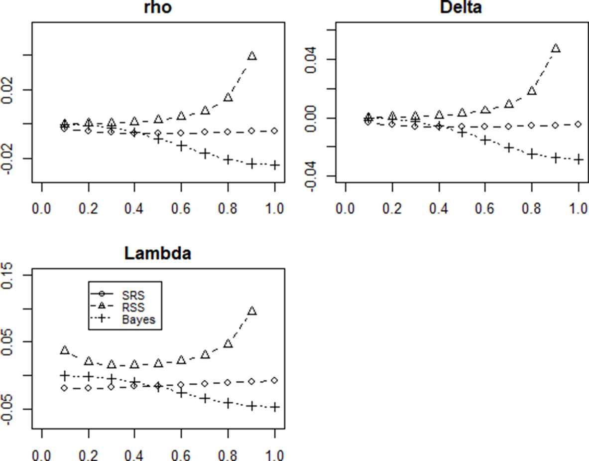
The bias estimates of overlap coefficients by R.
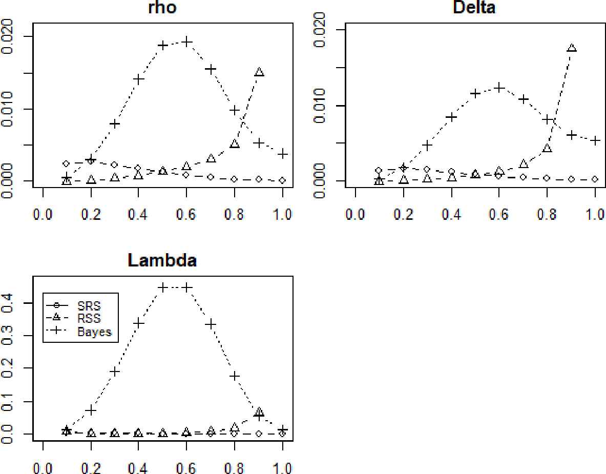
The Mean Squared Error (MSE) estimates for overlap coefficients by R.
7. REAL DATA APPLICATION
As applications, considers the dataset discussed by Proschan [19]. The data of 30 and 12 successive failure time intervals (in hours) of the air-conditioning system of jet plane, Plane 8044 and Plane-7912, for fitting to Lomax distribution (Gupta et al. [20]). The inverse Lomax random variable (
Plane 8044:
Plane 7912:
Fitting both data sets to inverse Lomax distribution with parameters
| 0.011 | 0.060 | 0.012 | 0.055 | 0.228 | 0.046 | 0.047 | 0.220 | 0.040 | |
| 0.004 | 0.0003 | 0.0001 | 0.0015 | 0.007 | 0.001 | 0.022 | 0.018 | 0.030 | |
| (0.991, 1.0) | (0.915, 1.0) | (0.990, 1.0) | (0.803, 0.932) | (0.799, 0.999) | (0.798, 0.921) | (0.763, 1.0) | (0.94, 1.0) | (0.70, 1.0) | |
Results based on the real data.
Since the confidence interval obtained by
8. CONCLUSION
In this paper we considered three measures of overlap, namely Matusia's measure
CONFLICTS OF INTEREST
The authors declare that there are no conflicts of interest regarding the publication of this paper.
AUTHORS' CONTRIBUTIONS
All authors have read and agreed to the published version of the manuscript.
ACKNOWLEDGMENTS
The authors would like to thank the Editor in Chief of JSTA and the anonymous referees for many helpful comments and suggestions.
REFERENCES
Cite this article
TY  - JOUR
AU  - Hamza Dhaker
AU  - El Hadji Deme
AU  - Salah El-Adlouni
PY  - 2021
DA  - 2021/01/15
TI  - On Inference of Overlapping Coefficients in Two Inverse Lomax Populations
JO  - Journal of Statistical Theory and Applications
SP  - 61
EP  - 75
VL  - 20
IS  - 1
SN  - 2214-1766
UR  - https://doi.org/10.2991/jsta.d.210107.002
DO  - 10.2991/jsta.d.210107.002
ID  - Dhaker2021
ER  -