
Modified Maximum Likelihood Estimations of the Epsilon-Skew-Normal Family
- DOI
- 10.2991/jsta.d.201208.001How to use a DOI?
- Keywords
- Asymmetry; EM-algorithm; Epsilon-skew-normal; Maximum likelihood estimates; Two-piece distributions
- Abstract
In this work, maximum likelihood (ML) estimations of the epsilon-skew-normal (ESN) family are obtained using an EM-algorithm to modify the ordinary estimation already used and solve some of its problems within issues. This family can be used for analyzing the asymmetric and near-normal data, so the skewness parameter epsilon is the most important parameter among others. We have shown that the method has better performance compared to the method in G.S. Mudholkar, A.D. Hutson, J. Statist. Plann. Infer. 83 (2000), 291–309, especially in the strong skewness and small samples. Performances of the proposed ML estimates are shown via a simulation study and some real datasets under some statistical criteria as a way to illustrate the idea.
- Copyright
- © 2020 The Authors. Published by Atlantis Press B.V.
- Open Access
- This is an open access article distributed under the CC BY-NC 4.0 license (http://creativecommons.org/licenses/by-nc/4.0/).
1. INTRODUCTION
The importance of the asymmetric distributions in various applications such as meteorology, physics, economics, geology, etc., has been rapidly increasing. Also, the asymmetric distributions which contain famous distributions in the symmetric cases, such as normal distribution, are more important among all others. The epsilon-skew-normal (ESN) distribution which was introduced by Refs. [1–6], is a flexible family to model the asymmetry data and statistical models. The ESN parameters maximum likelihood (ML) estimates were found by Refs. [3,7], and their Bayesian estimates were studied by Ref. [8] as well as Ref. [9].
The classical ML estimates of this family and its application on some statistical models (as regression model by Ref. [7]; time series model by Ref. [10]; Tobit regression by Ref. [11]) were performed by an especial approach which ordered the data. Applying the variations of each produced segment and three possible likelihood function forms as well as their proposed estimates, the one with higher likelihood values was chosen as the approximation of the ML estimates (see e.g. Ref. [12]). But, there exist some problematic issues on this method, e.g., in the strong asymmetry, in the small samples, and the right/left half-normal distribution estimates in which there are not any real distributions. We have focused on an especial mixture of two right/left half-normal distributions which lead to ESN family, and have used an EM-algorithm to obtain the ML estimates of the model parameters. In addition, we have shown the modifications of the proposed ML estimates without the maintained issues (see, e.g., Ref. [13]).
The rest of this paper is organized as follows: Some properties of the ESN family and ordinary method of finding the ML estimates are considered in Section 2. The new approach of finding the ML estimates based on the mixture distributions are provided in Section 3. In Section 4, in order to show the performance of the proposed methodology, some simulation studies are provided which are later used to some real dataset. Finally, the conclusion is given in Section 5.
2. THE ESN FAMILY
The ESN distribution denoted by
Note that,
The mean and variance of the random variable
To see more statistical details of the ESN distribution, refer to the Refs. [1,3].
To obtain the ML estimates of the
3. ML ESTIMATES OF THE ESN PARAMETERS USING AN EM-ALGORITHM
3.1. ML Estimates
In fact the location-scale ESN distribution is the reparameterization of a mixture of left- and right half-normal (RHN) densities with special component probabilities as follows:
By using an EM-algorithm to obtain the
The conditional expectation of latent variables is
E-Step:
M-steps:
M-step 1: Update
M-steps 2–3: Update
3.2. Model Selection
In this paper we have just ESN family but with different numerical ML estimate types, therefore we compare different ESN distributions based on different estimated parameters (through mentioning different numerical approaches) to better fit on the simulated and real datasets. The Akaike information criteria (AIC; Ref. [19]) is in the form of
4. NUMERICAL STUDIES
In this section, we simulate the some strongly and weakly skewed ESN samples and use the proposed ML estimates (denoted by Pr-ML) to evaluate the ordinary ML estimates (denoted by Or-ML) which correspond to Refs. [1,3]. Then we apply the both ML estimation methods to some real datasets. The implementation of the necessary algorithms is based on the R software version 3.5.2 with a core i7 760 processor 2.8 GHz, and the relative tolerance of
4.1. Simulations
In this part, we consider 10,000 samples of size
| Parameters | ML | n = 50 |
n = 100 |
n = 250 |
|||
|---|---|---|---|---|---|---|---|
| Mean | SD | Mean | SD | Mean | SD | ||
| Or-ML | −0.1026 | 0.1637 | 0.0837 | 0.0936 | −0.0657 | 0.0746 | |
| Pr-ML | −0.1017 | 0.1726 | 0.0866 | 0.0894 | −0.0719 | 0.0563 | |
| Or-ML | 1.0258 | 0.0403 | 1.0137 | 0.0304 | 0.9846 | 0.0307 | |
| Pr-ML | 1.0144 | 0.0397 | 1.0003 | 0.0294 | 0.9930 | 0.0308 | |
| Or-ML | 0.0618 | 0.0106 | 0.0589 | 0.0095 | 0.0440 | 0.0082 | |
| Pr-ML | 0.0585 | 0.0098 | 0.0558 | 0.0094 | 0.0528 | 0.0080 | |
| Or-ML | 0.1134 | 0.2016 | 0.1037 | 0.1073 | 0.0589 | 0.0374 | |
| Pr-ML | 0.1076 | 0.2113 | 0.0937 | 0.0783 | 0.0593 | 0.0412 | |
| Or-ML | 1.0312 | 0.0553 | 1.0207 | 0.0494 | 1.0201 | 0.0365 | |
| Pr-ML | 1.0189 | 0.0388 | 1.0054 | 0.0307 | 1.0036 | 0.0340 | |
| Or-ML | −0.5303 | 0.0128 | −0.5203 | 0.0097 | −0.5176 | 0.0066 | |
| Pr-ML | −0.5274 | 0.0078 | −0.5148 | 0.0071 | −0.5104 | 0.0061 | |
| Or-ML | 0.1981 | 0.1803 | −0.1037 | 0.1006 | 0.0579 | 0.0793 | |
| Pr-ML | 0.1805 | 0.1891 | −0.0937 | 0.0954 | 0.0667 | 0.0534 | |
| Or-ML | 1.0537 | 0.0683 | 1.0365 | 0.0546 | 1.0311 | 0.0397 | |
| Pr-ML | 1.0203 | 0.0442 | 1.0112 | 0.0410 | 1.0103 | 0.0385 | |
| Or-ML | 0.9204 | 0.0983 | 0.9048 | 0.0784 | 0.8910 | 0.0719 | |
| Pr-ML | 0.8399 | 0.0068 | 0.8401 | 0.0065 | 0.8411 | 0.0059 | |
| Or-ML | 0.1907 | 0.1887 | 0.1117 | 0.0936 | 0.0794 | 0.0864 | |
| Pr-ML | 0.1870 | 0.1804 | 0.0946 | 0.0911 | 0.0642 | 0.0570 | |
| Or-ML | 1.0497 | 0.0702 | 1.0405 | 0.0528 | 1.0352 | 0.0401 | |
| Pr-ML | 1.0286 | 0.0513 | 1.0201 | 0.0465 | 1.0112 | 0.0389 | |
| Or-ML | −0.9987 | 0.0057 | −0.9902 | 0.0102 | −0.9893 | 0.0096 | |
| Pr-ML | 0.9601 | 0.0113 | −0.9578 | 0.0094 | −0.9523 | 0.0075 | |
ESN, epsilon-skew-normal; ML, maximum likelihood; Pr-ML, proposed maximum likelihood; Or-ML, ordinary maximum likelihood.
Mean and standard deviations (SDs) of the 10,000 times Or-ML and Pr-ML estimates of the ESN distribution.
4.2. Applications
In this section, considering four various real datasets, we show the performance of the proposed Pr-ML estimates in applications. All of ESN parameters estimates and criteria are given in Table 2, and the fitted ESN densities based on the two approaches Pr-ML and Or-ML estimates are curved on the histograms of the mentioned datasets in Figure 1.
| Data | ML | Parameter |
Criteria |
||||
|---|---|---|---|---|---|---|---|
| AIC | K-S | A-D | |||||
| 1st Data | Or-ML | 0.0246 | 1.8938 | −1.0000 | 2108.798 | 0.0417 | 1.4202 |
| Pr-ML | 0.0246 | 1.8939 | −1.0000 | 2108.841 | 0.0416 | 1.4169 | |
| 2nd Data | Or-ML | 43.9999 | 55.2043 | −0.9384 | 6317.510 | 0.1047 | 12.8735 |
| Pr-ML | 40.9727 | 55.5884 | −0.9569 | 6291.083 | 0.0945 | 8.3241 | |
| 3rd Data | Or-ML | 0.9790 | 0.2994 | −0.0578 | 3643.910 | 0.0551 | 62.1247 |
| Pr-ML | 1.1461 | 0.2919 | 0.3249 | 3015.756 | 0.0343 | 13.3147 | |
| 4th Data | Or-ML | 4.4999 | 0.2726 | −0.6772 | 4167.713 | 0.3357 | 592.7232 |
| Pr-ML | 4.2438 | 0.3771 | −0.6155 | 893.682 | 0.0796 | 4.3623 | |
ESN, epsilon-skew-normal; ML, maximum likelihood; Pr-ML, proposed maximum likelihood; Or-ML, ordinary maximum likelihood; K-S, Kolmogorov–Smirnov; A-D, Anderson–Darling.
The Or-ML and Pr-ML estimates of the fitted ESN distributions on four real datasets.
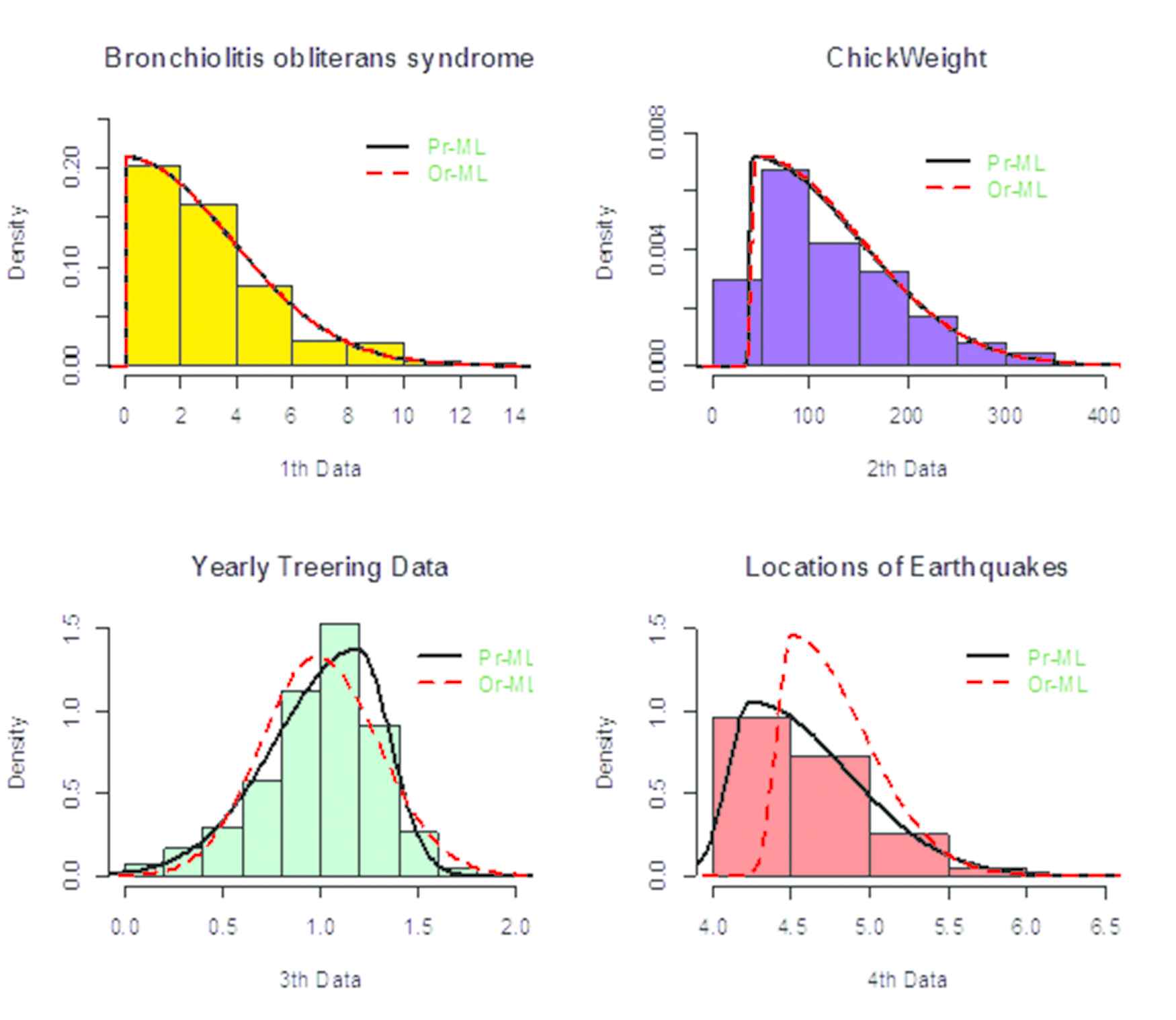
Histograms of the real datasets with the curved fitted epsilon-skew-normal (ESN) densities based on the proposed maximum likelihood (Pr-ML) and ordinary maximum likelihood (Or-ML) estimates.
The first dataset is corresponds to the “Tstop” component of the “Bronchiolitis obliterans syndrome after lung transplants” called “bosms3” and available in the “flexsurv” package of R software. Both Pr-ML and Or-ML estimates satisfy the purely skewed right half-normal (
The second dataset is corresponds to the “weight” component of the “Weight versus age of chicks on different diets” called “ChickWeight” and it is available in the “datasets” package of R software. In this case, although the Or-ML and Pr-ML estimates are close (see, e.g., the Table 2 and top-right of the Figure 1), but all of the criteria prefer the fitted ESN distribution based on the Pr-ML to Or-ML estimates.
The third dataset is corresponds to the “Yearly Treering Data” called “treering” and it is available in the “datasets” package of R software. In this case, all of the criteria strongly prefer the fitted ESN distribution based on the Pr-ML to Or-ML estimates (see, e.g., the Table 2 and bottom-left of the Figure 1).
The fourth dataset is corresponds to the “mag” component of the “Locations of Earthquakes off Fiji” called “quakes” and it is available in the “datasets” package of R software. In this case, also all of the criteria strongly prefer the fitted ESN distribution based on the Pr-ML to Or-ML estimates (see, e.g., the Table 2 and bottom-right of the Figure 1).
5. CONCLUSION
We have proposed and implemented an EM-type algorithm to estimate the well-known ESN family parameters by applying the special stochastic representation. The proposed estimation methodology has better ESN distribution fitting, especially in the strong skewness. The performance of the proposed methodology is illustrated using the simulation studies and four real datasets. The performances of the ESN family have shown on many statistical models to cover the asymmetry, e.g., Refs. [3,7,10]. In fact, this methodology can be affronted on them to modify their parameter estimations.
CONFLICTS OF INTEREST
The authors declare that there are no conflicts of interest regarding the publication of this paper.
AUTHORS' CONTRIBUTIONS
All authors have read and agreed to the published version of the manuscript.
FUNDING STATEMENT
There is no funding of this paper.
ACKNOWLEDGMENTS
We would like to express our very great appreciation to editor and reviewer(s) for their valuable and constructive suggestions during the planning and development of this research work.
REFERENCES
Cite this article
TY  - JOUR
AU  - Parichehr Jamshidi
AU  - Mohsen Maleki
AU  - Zahra Khodadadi
PY  - 2020
DA  - 2020/12/14
TI  - Modified Maximum Likelihood Estimations of the Epsilon-Skew-Normal Family
JO  - Journal of Statistical Theory and Applications
SP  - 481
EP  - 486
VL  - 19
IS  - 4
SN  - 2214-1766
UR  - https://doi.org/10.2991/jsta.d.201208.001
DO  - 10.2991/jsta.d.201208.001
ID  - Jamshidi2020
ER  -