Log-Kumaraswamy Weibull regression model; Moments; Maximum likelihood estimation
Abstract
This paper investigates the potential usefulness of the transmuted Kumaraswamy Weibull distribution by using quadratic rank transmutation map technique for modelling reliability data. Some structural properties of the transmuted Kumaraswamy Weibull distribution are discussed. We propose a location-scale regression model based on the transmuted log-Kumaraswamy Weibull distribution for modelling survival data. We discuss estimation of the model parameters by the method of maximum likelihood and provide two applications to illustrate the potentiality of the proposed family of lifetime distributions.
The Weibull distribution is a very popular distribution, which was initially developed by the Swedish physicist Waloddi Weibull in 1937 for modelling breaking strength of materials data. The Weibull distribution is widely used statistical model for studying the life-testing problems. In some cases, the Weibull distribution is proved to be a good alternative to the log-normal, gamma and generalized exponential distributions. The Weibull distribution is well- appreciated model in the statistics literature for explaining bathtub-shaped curve. The Weibull distribution having exponential and Rayleigh as special sub-models for modelling lifetime data and for modelling phenomenon with monotone failure rates. The statistics literature in distribution theory has growing interest for studying life-testing problems. In the last few years many new families of lifetime distributions have been proposed based on the modification of the Weibull distribution for explaining real-world scenarios. The exponentiated Weibull (EW) distribution was introduced by Mudholkar and Srivastava [1], the additive Weibull distribution presented by Xie and Lai [2], the extended Weibull distribution studied by Xie et al. [3], the modified Weibull (MW) distribution proposed by Lai et al. [4], Kumaraswamy Weibull distribution proposed by Cordeiro et al. [5]. The five parameters Kumaraswamy MW distribution proposed by Cordeiro et al. [6]. Aryal and Tsokos [7] offered the transmuted Weibull distribution by using the quadratic rank transmutation map method proposed by Shaw and Buckley [8]. Khan and King [9] introduced and studied some mathematical properties of the transmuted MW distribution. Khan et al. [10] studied the flexibility of the transmuted Inverse Weibull distribution with various structural properties through an application to survival data. More recently Khan et al. [11,12] studied the transmuted generalized exponential and transmuted Weibull distributions with covariates regressing modelling to analyze survival data. Merovci [13,14] proposed the transmuted Rayleigh distribution and transmuted generalized Rayleigh distribution for modelling lifetime data. Yuzhu et al. [15] studied the transmuted linear exponential distribution with an application to reliability data. The density function of Weibull distribution with two parameters given by
gx;η,θ=θηθxθ−1exp−ηxθ,x>0(1)
The cumulative distribution function corresponding to (1) is given by
Gx;η,θ=1−exp−ηxθ.(2)
Here η>0 is the scale parameter and θ>0 is the shape parameter of the Weibull distribution. In this research, we investigate the potential usefulness of the transmuted Kumaraswamy Weibull distribution, which contains several well-known distributions. As the special sub-models, such as transmuted Weibull distribution, transmuted Rayleigh distribution, Kumaraswamy Weibull distribution, transmuted Kumaraswamy Rayleigh distribution, among several others. The proposed family of distributions can be used effectively for modelling survival data, since it accommodates monotonically increasing, decreasing and constant bathtub-shaped hazard rate functions. The transmuted Kumaraswamy Weibull distribution is more flexible for modelling bathtub-shaped hazard function than the Kumaraswamy Weibull distribution. More recently, Khan et al. [16] introduced the transmuted Kumaraswamy G family of lifetime distribution with two applications of Aircraft windshield data sets. For an arbitrary baseline cdf Gx,ξ, we define the TKw-G distribution by using the pdf fx,ξ and cdf Fx,ξ are given by
respectively, If X is a random variable with pdf (3), then we write X~TKw-Gx;α,β,λ,ξ, where α and β are the shape parameters, λ is the transmuting parameter, ξ is the parameters vector of the baseline model and gx,ξ is the derivative of Gx,ξ. For α=β=1 the proposed family of distribution reduces to the transmuted family distributions introduced by Bourguignon et al. [17]. By substituting λ=0 in Equation (3), we obtain the Kw-G family of distribution proposed by Cordeiro and de Castro [18].
The rest of the paper is outlined as follows: In Section 2, we define the TKwW distribution and discussed some special cases of this model and quantiles. In Section 3, we formulate the expression of moments, moment-generating function and incomplete moments. Maximum likelihood estimation of the model parameters is discussed in Section 4. In Section 5, we discuss the transmuted log-Kumaraswamy Weibull distribution and derive its moments. Section 6 illustrated two applications of the TKw-Weibull family of distributions, followed by concluding remarks.
2. TRANSMUTED KUMARASWAMY WEIBULL DISTRIBUTION
A random variable X has the TKw-Weibull distribution with parameters α,β,η,θ>0 and |λ|≤1, x>0. The density function of the TKw Weibull distribution (see Khan et al. [16]), given by
Here α,β,θ control the shape of the distribution, η controls the scale of the distribution and λ is the transmuting parameter, which provides the extra flexibility in the new extended model. If X is a random variable having the TKw Weibull distribution, we write X~TKwWx;α,β,η,θ,λ. The reliability function (RF), hazard function (HF) and cumulative hazard function (CHF) corresponding to (5) are given by
The qth quantile xq of the TKw Weibull random variable is given by
xq=1η−log1−1−1−1+λ−1+λ2−4λq2λ1β1α1θ,0<q<1(9)
The TKw Weibull model contains as special cases seventeen lifetime distributions are displayed in Figure 1. The TKwR distribution is the special case of the TKwW distribution when shape parameter θ=2. The Kw Weibull distribution proposed by Cordeiro et al. [5], is the special case of the TKwW distribution, when λ=0. If θ=2 in addition to λ=0, it reduces to the Kw Rayleigh distribution. The transmuted exponentiated Weibull (TEW) model is also the special case of the TKwW distribution when β=1. If α=1 in addition to β=1 it reduces to the transmuted Weibull distribution proposed by Aryal and Tsokos [7].
Figure 1
Relationships of the TKw Weibull sub-models.
For α=β=1 and θ=2, the TKwW distribution reduces to the transmuted Rayleigh distribution proposed by Merovci [13]. Figure 2 shows some possible shapes of probability density functions of the TKwW distribution for some selected values of parameters. The visualizations in Figure 3 demonstrates some promising shapes of the hazard functions for the TKwW distribution with some selected values of parameters. The hazard function of the TKw Weibull distribution has the monotone decreasing and increasing, U shapes and J shapes bathtub hazard rate functions. The quantile function of the Tkw Weibull distribution is useful for obtaining the percentile life. Table 1 shows the quartile values of the Tkw Weibull distribution for some selected values of parameters. By substituting q=0.5 in Equation (9) we obtain the median of the Tkw Weibull distribution. Equation (9) is also useful for generating random numbers for the Tkw Weibull distribution. The Tkw Weibull distribution contains as special sub-models some new lifetime distributions.
Figure 2
Plots of the TKw Weibull Probability density function (PDF) for some parameter values.
Figure 3
Plots of the TKw Weibull Hazard function (HF) for some parameter values.
The four-parameter transmuted Kumaraswamy Rayleigh (TKw-R) distribution is the special case of the TKw Weibull distribution by substituting θ=2 in Equation (5). If λ=0 it corresponds to the Kw Rayleigh distribution. If α=1 and β=1, it reduces to the transmuted Rayleigh distribution proposed by Merovci [13]. If α=β=1 in addition to λ=0, the TKw-R distribution simplifies to the Rayleigh distribution introduced by Lord Rayleigh [19].
The four-parameter transmuted Kumaraswamy exponential (TKw-E) distribution is the special case of the TKw Weibull distribution by substituting θ=1 in Equation (5). If λ=0 it corresponds to the Kw exponential distribution. If β=1, it reduces to the transmuted generalized exponential distribution proposed by Khan et al. [11]. If α=1 and β=1, it reduces to the transmuted exponential distribution proposed by Owoloko et al. [20].
The four-parameter TEW distribution is the special case of the TKw Weibull distribution by substituting β=1 in Equation (5). If λ=0 it corresponds to the Kw Weibull distribution proposed by Cordeiro et al. [5]. If λ=0 in addition to β=1, it reduces to EW distribution proposed by Mudholkar and Srivastava [1]. If α=1, it reduces to the transmuted Weibull distribution proposed by Aryal and Tsokos [7].
3. STATISTICAL PROPERTIES
This section presents the moments, moment-generating function and incomplete moments of the transmuted TKwW distribution.
Theorem 1.
IfXhas theTKwWdistribution with|λ|≤1, then thekthmoment ofXsayμ´kis given as follows:
The values of the moments can be calculated numerically by the Monte Carlo method with respect to the integral using R or SAS languages. Table 2 shows the moments and Table 3 displays the mean, variance, coefficient of variation, coefficient of skewness and coefficient of kurtosis measures of the TKwW distribution.
Estimates
α
β
η
θ
λ
μ´1
μ´2
μ´3
μ´4
1
1.5
1
1.5
−1
0.9438
1.1116
1.5555
2.5073
−0.50
0.8163
0.9025
1.2222
1.9340
0.50
0.5614
0.4842
0.5555
0.7875
1
0.4339
0.2751
0.2222
0.2143
1
2
1.5
2.5
−1
0.5568
0.3389
0.2223
0.1555
−0.50
0.5025
0.2883
0.1822
0.1243
0.50
0.3940
0.1871
0.1019
0.0619
1
0.3397
0.1365
0.0618
0.0307
2
3
1.5
3.5
−1
0.6400
0.4182
0.2787
0.1892
−0.50
0.6074
0.3810
0.2457
0.1624
0.50
0.5422
0.3065
0.1797
0.1089
1
0.5096
0.2693
0.1468
0.0822
2
3.6
2
5
−1
0.4735
0.2265
0.1094
0.0533
−0.50
0.4561
0.2114
0.0994
0.0473
0.50
0.4213
0.1812
0.0794
0.0354
1
0.4039
0.1661
0.0694
0.0294
Table 2
Moments of the TKw Weibull distribution with some parameter values.
Estimates
α
β
η
θ
λ
Mean
Var
CV
CS
CK
1
1.5
1
1.5
−1
0.9438
0.2208
0.4979
0.8624
4.0111
−0.50
0.8163
0.2361
0.5953
0.8709
3.9356
0.50
0.5614
0.1690
0.7323
1.3509
5.5197
1
0.4339
0.0868
0.6791
1.0741
4.3863
1
2
1.5
2.5
−1
0.5568
0.0288
0.3052
0.2948
2.9411
−0.50
0.5025
0.0357
0.3765
0.2003
2.7982
0.50
0.3940
0.0318
0.4531
0.5404
3.2294
1
0.3397
0.0211
0.4276
0.3565
2.8892
2
3
1.5
3.5
−1
0.6400
0.0086
0.1449
0.0551
2.4316
−0.50
0.6074
0.0121
0.1808
−0.2839
3.3906
0.50
0.5422
0.0125
0.2064
−0.0428
3.3383
1
0.5096
0.0096
0.1923
−0.2417
2.7453
2
3.6
2
5
−1
0.4735
0.0023
0.1012
−0.2154
−2.4033
−0.50
0.4561
0.0034
0.1273
−0.4911
−0.8445
0.50
0.4213
0.0037
0.1445
−0.2769
3.9478
1
0.4039
0.0029
0.1348
−0.5126
2.1183
Table 3
Moments based measures of the TKw Weibull distribution.
Theorem 2.
IfXhas theTKwWdistribution with|λ|≤1, then the moment generating function ofX, MXtis given as follows:
The first incomplete moment of theTkwWeibull distribution can be obtained from (14) by substitutingk=1,is very useful measure for Bonferroni and Lorenz curves, mean residual life and for mean waiting time can be defined as
Consider the random samples x1,x2,…,xn consisting of n observations from the TKwWx;α,β,η,θ,λ distribution then we apply the maximum likelihood estimation for estimating the model parameters based on complete samples. The log-likelihood function L=lnL of (5) is given by
The log-likelihood function of the model parameters can be estimated by using the R package [21] or by solving the nonlinear log-likelihood equations obtained by differentiating Equation (16). For the interval estimation and hypothesis testing, we required the observed information matrix. All the second- order derivatives exist for the five parameters TKwW distribution. Thus, we have the asymptotic distribution defined as
α^,β^,θ^,η^,λ^T~N5α,β,θ,η,λT,kϑ−1,
where Kϑ is the 5×5 the expected unit information matrix
where kϑiϑj=∂2L/∂ϑiϑj,i,j=1,2,3,4,5. The asymptotic multivariate normal distribution can be used to construct the confidence intervals for each parameter. An asymptotic confidence interval for significance level γ for each parameter ϑr can be estimated as
ACIr=ϑ^r−Zγ/2−kr,rϑ^,ϑ^r+Zγ/2−kr,rϑ^,
where kr,r−1ϑ^ is the rth diagonal element of the inverse of observed information matrix kϑ^ and Zγ/2 is the 1−γ% quantile of the standard normal distribution.
5. TRANSMUTED LOG-KUMARASWAMY WEIBULL DISTRIBUTION
In the context of the survival studies, many new lifetime distributions have been developed for studying time to event data with covariates regression modelling. The location-scale regression models with covariates has a rich tradition in survival analysis and commonly used in clinical trials. Survival models provide more understanding of time to event data by allowing more flexible formulation with precise and informative conclusion. In this section, we examine statistical inference aspect and modelling a new regression using the logarithm of the transmuted Kumaraswamy Weibull distribution. The modification in the distribution under study leads to the location-scale regression model for fitting headache relief patient's data. If X is a random variable having the transmuted Kumaraswamy Weibull distribution, then Y=logX has the transmuted log-Kumaraswamy Weibull distribution. The density of Y, parameterize in terms of η=exp−μ and θ=1/σ, hence the density function of Y is given by
where −∞<Y<∞, −∞<μ<∞, with |λ|≤1, and α,β,σ>0. If Y has the transmuted log- Kumaraswamy Weibull distribution, then it is denoted by Y~TLKwWy;α,β,μ,σ,λ. The greater flexibility of the proposed model to fit survival data is due to the different forms of the density function for some selected values of parameters are displayed in Figure 4. The log-Kumaraswamy Weibull distribution is the special case of the transmuted log-Kumaraswamy Weibull distribution when the transmuting parameter λ=0. The standardized random variable Z=Y−μ/σ has the density function as
Figure 4
Plots of the transmuted log-Kumaraswamy Weibull distribution.
The proposed model reduces to the transmuted log-EW distribution, when β=1. If λ=0, in addition to β=1, the transmuted log-Kumaraswamy Weibull model becomes the log-EW distribution proposed by Hashimoto et al. [22].
The covariates vector is denoted by x=x1,x2,…,xmT associated with the ith response variable yi through regression model. Consider the re-parametrization for the covariates regression by taking scale parameter μ=xTβ which depends on the explanatory variable Y and the scale parameter μ depends on the matrix of the explanatory variable X in the TLKwW regression model. We assume that the lifespans of time to event data are independently distributed and also independent from censoring technique. Considering right censored lifetime data, we observe yi=minYi,Ci, where Yi is the lifetime and Ci is the censoring time, both for ith individual i=1,2,…,n.
Now we construct the linear regression model for the response variable yi|X based on the TLKwW regression model can be represented as
yi=XTθ+σzi,i=1,2,…,m,(21)
where θ=θ1,θ2,…,θmT, σ>0 and |λ|≤1 are the unknown parameters, XT=x1,…,xm is the vector of explanatory variables and the survival function of yi can be estimated as
Let F and C be the sets of individuals for which yi is the log-lifetime or log-censoring, respectively. The total log-likelihood function for the TLKwW regression model parameters Θ=α,β,σ,λ,θTT can be obtained from Equations (20) and (21) as
where zi=yi−XTθσ. Under the regularity conditions that are fulfilled in the boundary of the sample space for the parameter vector Θ, the asymptotic distribution of nΘ^−Θ is multivariate normal Nm+40,kΘ−1, where kΘ is the expected information matrix. For testing of hypothesis and confidence intervals estimates for α,β,σ,λ,θTT of the TLKwW regression model based on the asymptotic distribution is defined as
α^,β^,σ^,λ^,θ^TT~Nm+4α,β,σ,λ,θTT,k−1Θ^,
where KΘ^ is the m+4×m+4 observed information matrix.
The asymptotic multivariate normal Nm+40,kΘ^−1 distribution can be used to construct the confidence intervals for each parameter Θ.1001−γ% asymptotic confidence intervals for each parameter Θ can be estimated by using the well-known procedure in statistics literature. Further we can construct likelihood ratio statistics for comparing sub-models for the TLKwW distribution by using the values of log-likelihood.
Theorem 4.
IfYhas aTLKwWy;α,β,μ,σ,λdistribution with|λ|≤1, then thekthmoment ofY,sayμ´kis given by
In this section, we present the usefulness of the TKwW distribution and TLKwW regression model applied to two real data sets.
6.1. Application 1: Fatigue Life of Aluminium Data
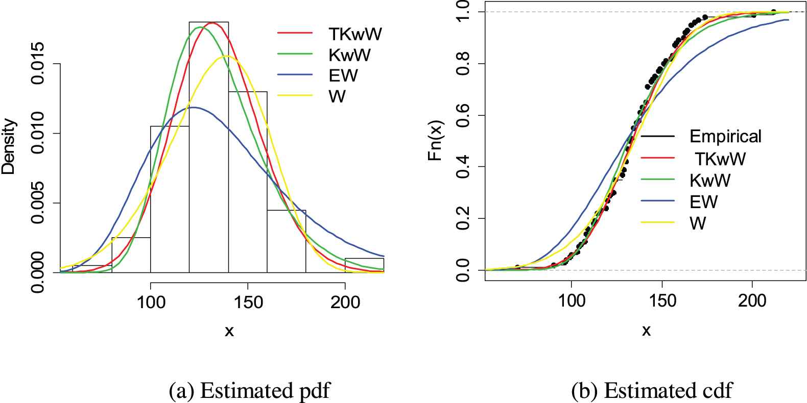
In this section, we provide an application to illustrate the flexibility of the Tkw Weibull distribution and compare this model with four different lifetime distributions for data modelling. The data set refers to the fatigue life of 6061-T6 aluminium coupons cut parallel with the direction of rolling and oscillated at 18 cycles per second. The data set consists of 101 observations with maximum stress per cycle 31,000 psi, which were originally reported by Birnbaum and Saunders [23]. We fitted five distributions namely: transmuted Kumaraswamy Weibull distribution [16], Kumaraswamy transmuted Weibull distribution [24], Kumaraswamy Weibull distribution [5], EW [1] and Weibull distribution [25]. The model's parameters are estimated by the method of maximum likelihood and four goodness of-fit statistics are used to compare the transmuted Kumaraswamy Weibull model with other four distributions. The Maximum Likelihood Estimation (MLEs) of the unknown parameter(s) with their corresponding standard errors in parenthesis and the corresponding Akaike information criteria (AIC) for the fitted models are listed in Table 4. Furthermore, we applied the K-S test, the Cramér-von Mises and Anderson-Darling goodness of-fit statistics in order to verify, which model provides the better estimate for the fatigue life of aluminium data. Table 5 shows that the TkwW distribution has the smallest values of these statistics; therefore the TkwW model can be chosen as the best model among the four competitive models. Finally, in order to access whether the TkwW distribution is appropriate for the fatigue life of aluminium data, plots of the fitted pdfs and cdfs of the TkwW, kwTW, kwW, EW and W distributions are displayed in Figure 5.
Model
Parameter Estimates
AIC
α^
β^
η^
θ^
λ^
TkwW
11.0468
4.8596
0.0104
1.6159
0.3111
914.73
(2.0429)
(12.9815)
(0.0011)
(0.5588)
(0.4381)
kwTW
28.4867
5.6224
1.1055
55.5826
0.0001
914.83
(34.8781)
(1.5020)
(0.3640)
(41.4296)
(0.0024)
kwW
19.1444
0.6425
0.0139
2.2342
–
917.71
(41.9197)
(1.1386)
(0.0085)
(2.3567)
EW
19.5586
1.2631
0.0070
–
–
943.45
(3.6944)
(0.0272)
(0.0009)
W
–
143.315
5.9789
–
–
922.19
(2.5402)
(0.4173)
AIC, Akaike information criteria
Table 4
MLEs of the Parameters for fatigue life of aluminium data and the AIC measure.
Model
K-S Test
W
A
TkwW
0.0665
0.0445
0.3087
kwTW
0.0664
0.0473
0.3195
kwW
0.1003
0.1159
0.6749
EW
0.1411
0.0864
0.5154
W
0.0981
0.1404
0.9639
Table 5
The K-S test, Cramér-von Mises and Anderson-Darling goodness of-fit tests.
Figure 5
Fitted models for fatigue life of aluminium data.
It is believable that if the true lifetime distribution is a TkwW/kwW distribution for fitting the fatigue life of aluminium data. This is predictable and is completed as a validation check to ensure that the derived MLEs formulation for the TkwW distribution is consistent with the fatigue life of aluminium data. As expected, in Figure 5(a), which represents the case when the TkwW distribution fitted to the fatigue life of aluminium data, the TkwW fit (red) overlaps almost entirely with the original distribution of the fatigue life of aluminium data and is suggestive of a good fit. The kwW density (green) slightly deviates from the original distribution of the fatigue life of aluminium data. The same behavior is observed in Figure 5(b), where the TkwW distribution is a competing model for the fatigue life of aluminium data.
These fitted models indicate that the TkwW distribution is superior to the other four models in terms of data fitting. In the light of the above remarks, we conclude that the TkwW model has better relationship for the fatigue life of aluminium data. Throughout this research article, we conclude that the conventional lifetime distributions currently in use are not the best choice in many practical scenarios, therefore we provide an efficient alternative that can be directly implemented by introducing the transmuted parameter in the base model.
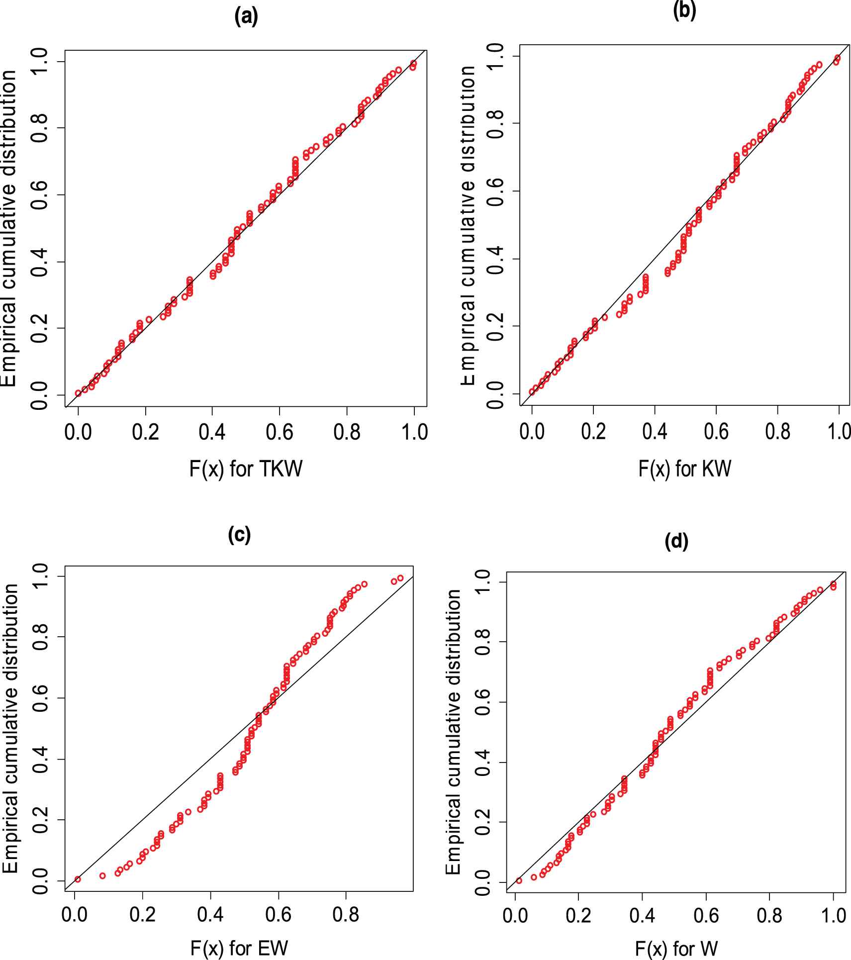
Figure 6 shows the PP-Plots of the TkwW, kwW, EW and W distributions used to compare the empirical cumulative distribution function of a data set with a specified theoretical cumulative distribution function and suggest that the TkwW distribution provides a better fit for the fatigue life of aluminium data.
Figure 6
P-P Plots of the TKW, KW, exponentiated Weibull (EW) and W models for fatigue life of aluminium data.
The Cramér-von Mises and Anderson-Darling goodness of-fit tests of the Kumaraswamy Weibull as a sub-model of the transmuted Kumaraswamy Weibull (TKW) suggests Kumaraswamy Weibull's (kW) inadequacy to describe the fatigue life of aluminium data. The K-S test and P-P plots (Figure 6) lead to the same conclusion for the TkwW fits, residuals of the TkwW PP fit lie closely to the unit-slope line, whereas residuals of the kwW fit deviate slightly from the unit-slope line in Figure 6(b). In view of the density and P-P Plots, it seems that the proposed model can be regarded as a suitable candidate model in the context of reliability analysis for modelling lifetime data.
6.2. Application 2: Headache Relief Data
This section demonstrates the applicability of the transmuted log-Kumaraswamy Weibull regression model, which adequately fits the observed data, discusses the clinical trials for thirty-eight headache relief patients' records (SAS/STAT 9.1. [26]) and identify the covariates are significantly associated with the response. We examine the utility of the proposed regression model by dividing data into two groups of equal size and different pain relievers assigned to each group. The outcome described is time in minutes until headache relief. The variable censor indicates whether relief was observed during the observation period (censor = 0) or whether the observation is censored (censor = 1). For regression model the experiment has been designed to evaluate the effect of headache relief (y) on groups x1 with censor observations. We consider the linear regression model fitted to the headache relief patients' data
yi=β0+β1xi1+σzi,
for i=1,2,…,38, where zi follows the TLKwW distribution given in Equation (18).
The maximum likelihood estimates of the model parameters are calculated with constraint |λ|≤1, using the general framework of the NLMixed in SAS [26]. Table 6 reports the MLEs, maximized log-likelihoods for the TLKwW, TLKwR and LKwW regression models with their corresponding standard errors in parenthesis. Considering the AIC, BIC and CAIC goodness of-fit measures of the fitted models displayed in Table 7, we find that the TLKwW regression model gives a better fit than the TLKwR and LKwW regression models.
The likelihood ratio test of the Kumaraswamy Weibull as a sub-model of the transmuted Kumaraswamy Weibull's inadequacy describe the headache relief patients' records data (Λ=6.6 on 1 df, with p-value = 0.0102 < 0.05). The AIC, BIC and CAIC goodness of-fit values are smaller for the TLKwW regression model than for the baseline model and sub-models lead to the same conclusion.
The likelihood ratio test is appealing because there is significant evidence in rejecting the null hypothesis. Based on this goodness of-fit measures, we conclude that the TLKwW regression model provides improved result for headache relief patients' data. Based on this ground, the proposed TLKwW regression model may play a very important role in modelling survival data.
Distribution
Parameter Estimates
α^
β^
θ^
λ^
b^0
b^1
TLKwW
4.3417
8.4464
1.7419
−0.5436
3.0135
0.0421
(20.5306)
(71.1515)
(6.3867)
(0.4795)
(0.9109)
(0.0657)
[<0.0021]
[0.5256]
TLKwR
1.5113
0.0859
–
−0.3851
1.5735
0.0456
(0.9044)
(0.0968)
(3.1683)
(0.0360)
(0.0222)
[<0.0001]
[0.0470]
LKwW
2.9024
0.1147
3.7569
–
2.4569
0.0223
(0.5377)
(0.0189)
(7.6547)
(0.9672)
(0.3542)
[<0.0040]
[0.3525]
Table 6
MLEs of the Parameters for fitted TLKwW, TLKwR, LKwW regression models to the headache relief data, with their corresponding SEs in parenthesis.
Distribution
AIC
Bayesian information criterion (BIC)
Consistent Akaikes Information Criterion (CAIC)
TLKwW
187.6
197.4
190.3
TLKwR
211.7
219.9
213.5
LKwW
189.0
197.5
190.9
AIC, Akaike information criteria.
Table 7
Goodness of-fit measures.
7. CONCLUDING REMARKS
In this paper, we propose the transmuted log-Kumaraswamy Weibull regression model and examine the performance of Tkw Weibull distribution. The transmuted Kumaraswamy Weibull distribution includes seventeen lifetime distributions as special sub-models. The analytical shapes of density and hazard functions are obtained for some selected choice of parameters. The Tkw Weibull model have flexible behavior for instantons failure rate function. Flexibility and usefulness of the proposed family of distributions are illustrated in two applications containing the fatigue life of aluminium coupons data and headache relief patients' data. We conclude that the Tkw Weibull distribution provides better estimates than the other competing models for the fatigue life of aluminium coupons data. Furthermore, we also introduced the transmuted log-Kumaraswamy Weibull distribution and obtained explicit expressions for its moments. Based on the Tkw Weibull distribution, we defined the TLKw Weibull regression model for studying time to event data. We have shown that new family of lifetime distributions perform better than the baseline distribution for explaining the real-world scenarios. We hope that the proposed extended family of distribution may attract wider applications for explaining the real-world phenomena.
CONFLICT OF INTEREST
The authors declare that they have no conflict of interest.
AUTHOR CONTRIBUTIONS
MSK, the principal investigator, conceptually developed the proposed distribution with related mathematical results, R and SAS codes for computation and drafted the manuscript. RK and ILH contributed in analysis and interpreted findings in discussion. All authors approved the final manuscript.
ACKNOWLEDGMENTS
The authors would like to thank the reviewers for their constrictive comments and suggestions, which certainly improved the quality and presentation of the paper.
8.W.T. Shaw and I.R.C. Buckley, The Alchemy of Probability Distributions: Beyond Gram–Charlier Expansions, and a Skew-Kurtotic Normal Distribution from a Rank Transmutation Map, 2009. Technical Report https://archive.org/details/arxiv-0901.0434
21.R Development Core Team, A Language and Environment for Statistical Computing, R Foundation for Statistical Computing, Vienna, Austria, 2013. http://www.R-project.org/
TY  - JOUR
AU  - Muhammad Shuaib Khan
AU  - Robert King
AU  - Irene Lena Hudson
PY  - 2020
DA  - 2020/10/29
TI  - Transmuted Kumaraswamy Weibull Distribution with Covariates Regression Modelling to Analyze Reliability Data
JO  - Journal of Statistical Theory and Applications
SP  - 487
EP  - 505
VL  - 19
IS  - 4
SN  - 2214-1766
UR  - https://doi.org/10.2991/jsta.d.201016.003
DO  - 10.2991/jsta.d.201016.003
ID  - Khan2020
ER  -