
Pranav Quasi Gamma Distribution: Properties and Applications
- DOI
- 10.2991/jsta.d.201202.001How to use a DOI?
- Keywords
- Quasi gamma distribution; Pranav distribution; Mixture models; Simulation study; Mixing parameter; Structural properties and maximum likelihood estimation
- Abstract
We have developed Pranav Quasi Gamma Distribution (PQGD) as a mixture of Pranav distribution
- Copyright
- © 2020 The Authors. Published by Atlantis Press B.V.
- Open Access
- This is an open access article distributed under the CC BY-NC 4.0 license (http://creativecommons.org/licenses/by-nc/4.0/).
1. INTRODUCTION
Continuous efforts have been made by researchers for many years to bring more and more flexibility in fitting probability models to real-life data. Flexibility can be introduced by generalizing the classical probability models or by mixing the two probability models. Need of mixture models arise when the population or distribution from which the data is obtained is a genuine mixture of k distinct populations or distributions and our aim is to estimate the proportions
A continuous r. v X will have a mixture distribution if its p.d.f
We have used mixture technique to obtain Pranav Quasi Gamma distribution (PQGD) in this paper.
2. PRANAV QUASI GAMMA DISTRIBUTION
A nonnegative r.v
In Equation (1)
And p.d.f of Quasi Gamma distribution
And corresponding c.d.f
Substituting values of
The graphs of p.d.f of PQGD are given in Figure 1a and 1b. These graphs show that for different parameter values indicating positively skewed nature of proposed model.
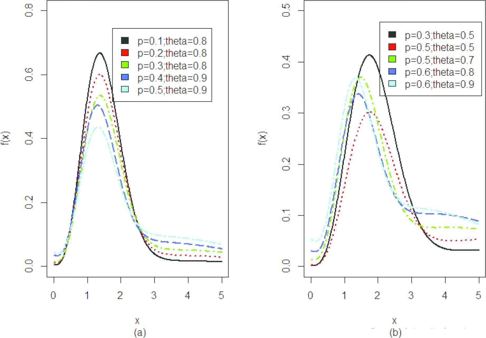
Graph of density function.
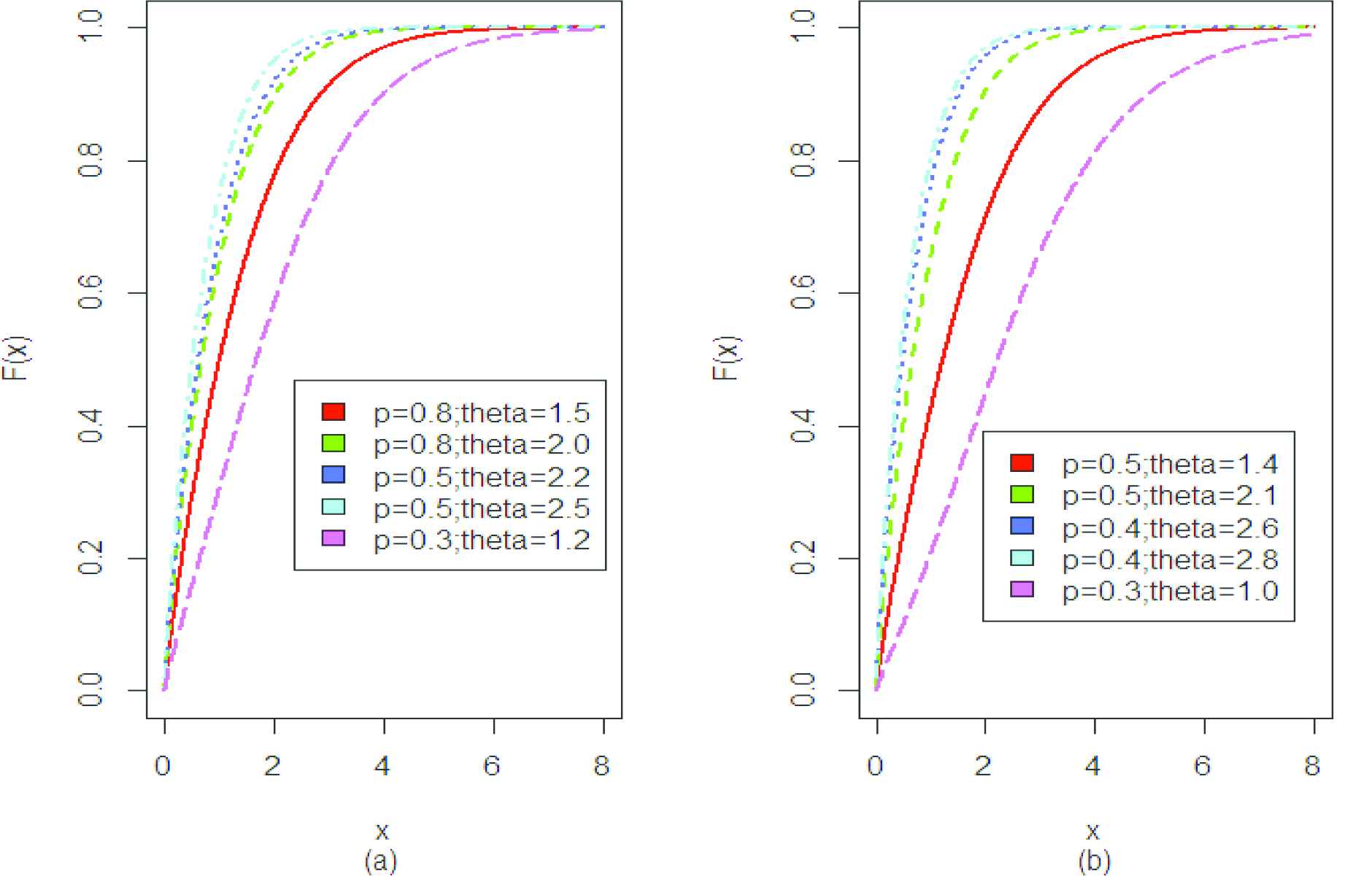
Graph of distribution function.
And the c.d.f of PQGD is found by using (3) and (5) and is given below
The above graphs represents the cumulative distribution function of PQGD.
3. RELIABILITY ANALYSIS
This different reliability measures are obtained in this particular area of paper. Expressions for survival function, failure rate and reverse failure rate of proposed PQGD are obtained in (8), (9), (10) respectively.
Figure 3a and 3b represent the survival function of PQGD. Figure 4 represents the hazard rate of PQGD which shows the flexibility of proposed model as the graph is inverted bathtub shaped. The hazard rate is of monotonic increasing as well as monotonic decreasing nature which shows the flexibility of proposed model.
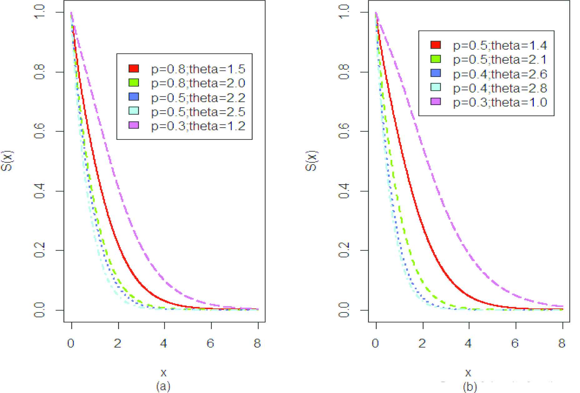
Graph of survival function.
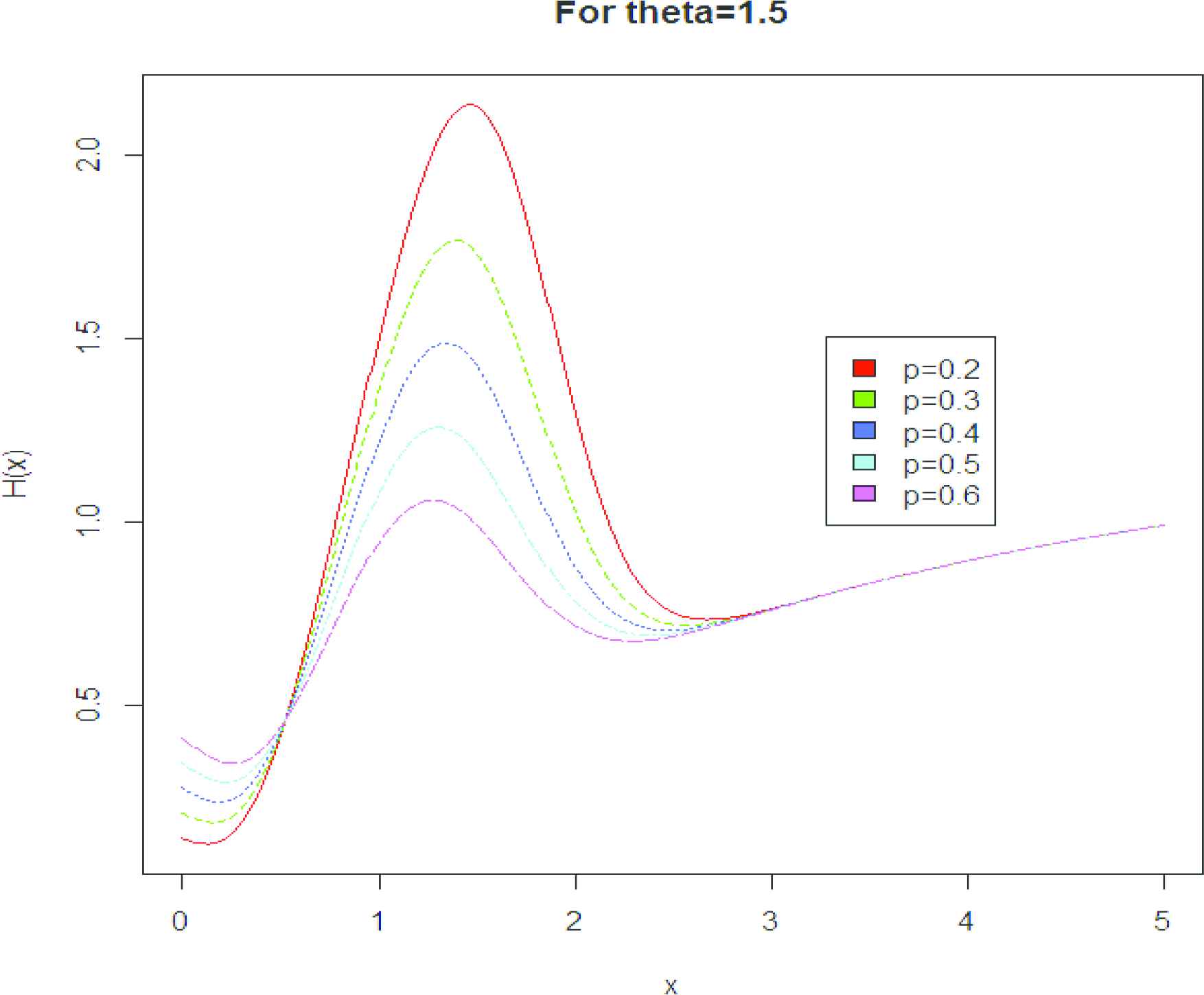
Graph of hazard function.
4. STATISTICAL PROPERTIES
Moments, mean deviation about mean, median characterize probability model among other properties. Here we have obtained these statistical properties for our proposed Pranav Quasi Gamma model.
4.1. Moments
Assuming
Put
Put
And variance of PQGD is
4.2. Average Deviation About Median and Arithmetic Mean of PQGD
We have derived the expressions for average deviation about median & arithmetic mean of PQGD in this area of paper.
Theorem 1:
If r.v X follows PQGD
Proof:
Average deviation about median
Using (6) we obtain
Using expressions (12), (13), (14), and (15) and expression for c.d.f (7) we obtain average deviation about median
5. ORDER STATISTICS OF PQGD
Assuming
Using the Equations (6) and (7), the probability density function of vth order statistics of PQGD is specified as
Then, the p.d.f of first order statistic
6. ESTIMATION OF PARAMETERS OF PQGD
Assuming
The log-likelihood function becomes
By partially differentiating (16) w. r. to θ and
MLEs of
7. SIMULATION STUDY
We have generated a data of 50 observations through R software by using inverse c.d.f technique from proposed model and we have obtained loss of information values AIC, BIC, AICC, and HQIC values for our model and its related models. We have also obtained the Shannon's entropy of our model and its related models. For testing the significance of mixing parameter p we used likelihood ratio (LR) statistic. In Table 1 estimates of parameters of fitted models along with model functions are given.
| Distribution | Parameter Estimates | Model Function |
|---|---|---|
| Quasi Gamma (QGD) | ||
| Pranav (PD) | ||
| Pranav Quasi Gamma (PQGD) |
ML estimates with standard errors in parenthesis, model function of proposed model, and its related models for simulated data of 50 observations.
In order to test the statistical significance of mixing parameter
| Distribution | AIC | BIC | AICC | HQIC | Shanon Entropy H(X) | Likelihood Ratio | |
|---|---|---|---|---|---|---|---|
| PQGD | 11.67180 | 27.3436 | 31.167 | 27.598 | 28.799 | 0.233 | 23.01 |
| QGD | 23.1788 | 48.3576 | 50.2696 | 48.440 | 48.44094 | 0.46 | |
| PD | 41.09660 | 84.1932 | 86.105 | 84.276 | 84.921 | 0.82 |
Model comparison and likelihood ratio statistic of proposed model and its related models.
Loss of information criteria's like AIC, BIC, AICC, and HQIC are computed along with measure of average uncertainty that is Shannon entropy H(X) for comparison of models fitted to data.
8. SPECIAL CASES
Case I: By putting
Case II: By putting
9. APPLICATIONS OF PQGD
We fitted PQGD and its related distributions to two real-life data sets and showed that our proposed model fits well to these data sets as compared to its related models.
Data Set 1: The data set given in Table 3 has been taken from Kotz and Johnson [11] and represents the survival times (in years) after diagnosis of 43 patients with some kind of leukemia.
| 0.019 | 0.129 | 0.159 | 0.203 | 0.485 | 0.636 | 0.748 | 0.781 |
|---|---|---|---|---|---|---|---|
| 0.869 | 1.175 | 1.206 | 1.219 | 1.219 | 1.282 | 1.356 | 1.362 |
| 1.458 | 1.564 | 1.586 | 1.592 | 1.781 | 1.923 | 1.959 | 2.134 |
| 2.413 | 2.466 | 2.548 | 2.652 | 2.951 | 3.038 | 3.6 | 3.655 |
| 3.745 | 4.203 | 4.690 | 4.888 | 5.143 | 5.167 | 5.603 | 5.633 |
| 6.192 | 6.655 | 6.874 |
Survival times (in years) after diagnosis of 43 patients with a certain kind of leukemia.
Data set 2: This data set given in Table 4 represents the Kevlar 49/epoxy strands failure times data (pressure at 90%) is taken from Makubate et al. [12].
| 0.01 | 0.01 | 0.02 | 0.02 | 0.02 | 0.03 | 0.03 | 0.04 | 0.05 | 0.06 | 0.07 |
|---|---|---|---|---|---|---|---|---|---|---|
| 0.07 | 0.08 | 0.09 | 0.09 | 0.10 | 0.10 | 0.11 | 0.11 | 0.12 | 0.13 | 0.18 |
| 0.19 | 0.20 | 0.23 | 0.24 | 0.24 | 0.29 | 0.34 | 0.35 | 0.36 | 0.38 | 0.40 |
| 0.42 | 0.43 | 0.52 | 0.54 | 0.56 | 0.60 | 0.60 | 0.63 | 0.65 | 0.67 | 0.68 |
| 0.72 | 0.72 | 0.72 | 0.73 | 0.79 | 0.79 | 0.80 | 0.80 | 0.83 | 0.85 | 0.90 |
| 0.92 | 0.95 | 0.99 | 1.00 | 1.01 | 1.02 | 1.03 | 1.05 | 1.10 | 1.10 | 1.11 |
| 1.15 | 1.18 | 1.20 | 1.29 | 1.31 | 1.33 | 1.34 | 1.40 | 1.43 | 1.45 | 1.50 |
| 1.51 | 1.52 | 1.53 | 1.54 | 1.54 | 1.55 | 1.58 | 1.60 | 1.63 | 1.64 | 1.80 |
| 1.80 | 1.81 | 2.02 | 2.05 | 2.14 | 2.17 | 2.33 | 3.03 | 3.03 | 3.34 | 4.20 |
| 4.69 | 7.89 |
Kevlar 49/epoxy strands failure times data (pressure at 90%).
R software version 3.5.3 [13] is used for analyzing the data. We have fitted QGD, PD, GD, WD, and PQGD to the data sets 1 and 2. The summary statistics of data sets 1 and 2 are displayed in Tables 5 and 6, MLEs of the parameters with standard errors in parenthesis, model functions are displayed in Table 7 and log-likelihood values, LR statistic, AIC, AICC, BIC, HQIC, and Shannon's entropy are displayed in Tables 8 and 9 respectively.
| Number of Observations | Minimum | First Quartile | Median | Mean | Third Quartile | Maximum |
|---|---|---|---|---|---|---|
| 43 | 0.019 | 1.212 | 1.923 | 2.534 | 3.700 | 6.874 |
Summary statistics of data set 1.
| Number of Observations | Minimum | First Quartile | Median | Mean | Third Quartile | Maximum |
|---|---|---|---|---|---|---|
| 101 | 0.010 | 0.240 | 0.800 | 1.025 | 1.450 | 7.890 |
Summary statistics of data set 2.
| Distribution | Parameter Estimates |
Model Function | |
|---|---|---|---|
| Data Set 1 | Data Set 2 | ||
| Quasi Gamma Distribution (QGD) | |||
| Pranav Distribution (PD) | |||
| Pranav Quasi Gamma Distribution (PQGD) | |||
| Gamma Distribution (GD) | |||
| Weibull distribution (WD) | |||
ML estimates with standard errors in parenthesis, model function of proposed model, and its related models for data set 1 and 2.
| Distribution | AIC | BIC | AICC | HQIC | Shanon Entropy H(X) | Likelihood Ratio | |
|---|---|---|---|---|---|---|---|
| PQGD | 80.07714 | 164.1543 | 167.6767 | 164.4543 | 165.4532 | 1.862 | 101.188 |
| QGD | 130.6714 | 263.3428 | 265.104 | 263.4404 | 263.9923 | 3.038 | |
| PD | 82.17808 | 166.3562 | 168.1174 | 166.4537 | 167.0056 | 1.911 | |
| GD | 82.12227 | 168.2445 | 171.7669 | 168.5445 | 169.5435 | 1.909 | |
| WD | 81.61015 | 167.2203 | 170.7427 | 167.5203 | 168.5192 | 1.897 |
Model comparison and Likelihood ratio statistic of proposed model and its related models for data set 1.
| Distribution | AIC | BIC | AICC | HQIC | Shanon Entropy H(X) | Likelihood Ratio | |
|---|---|---|---|---|---|---|---|
| PQGD | 102.8728 | 209.7456 | 214.9758 | 209.868 | 211.8629 | 1.018 | 506.18 |
| QGD | 355.9660 | 713.9321 | 716.5472 | 713.9725 | 714.9907 | 3.52 | |
| PD | 106.3711 | 214.7422 | 217.3573 | 214.7826 | 215.8008 | 1.05 | |
| GD | 102.9827 | 209.9655 | 215.2048 | 210.2421 | 212.2049 | 1.020 | |
| WD | 102.9768 | 209.9536 | 215.1839 | 210.0761 | 212.1071 | 1.019 |
Model comparison and Likelihood ratio statistic of proposed model and its related models for data set 2.
In order to test the statistical significance of mixing parameter
Loss of information criteria's like AIC, BIC, AICC, and HQIC are computed along with measure of average uncertainty that is Shannon entropy H(X) for comparison of models fitted to data.
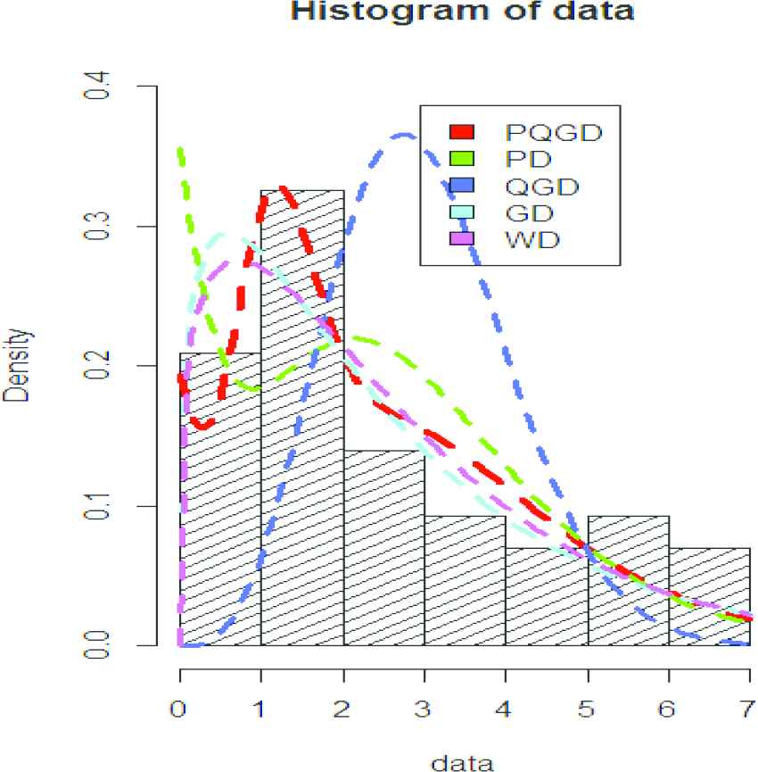
Curve fitting of data set 1.
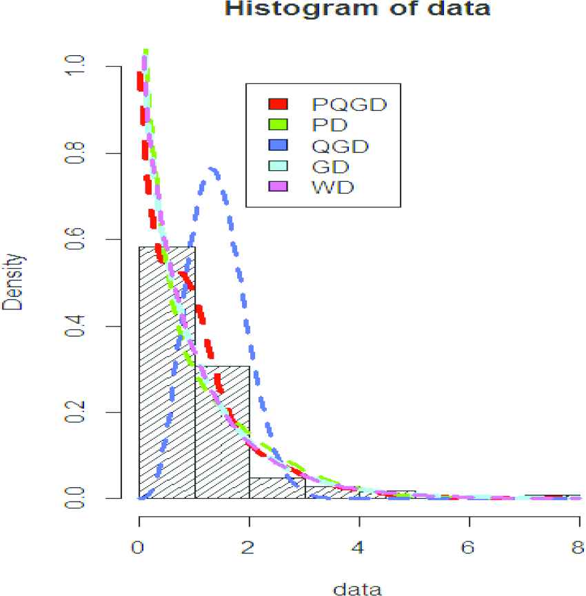
Curve fitting of data set 1.
10. CONCLUSION
We incorporated PQGD as a mixture of Pranav distribution and Quasi Gamma distribution. We obtained crucial properties of our proposed model. We carried out the simulation study and showed superiority of our model over its related models. We also obtained the estimates of our proposed model by using maximum likelihood method of estimation. Significance of mixing parameter has been tested. Finally we fitted our model and its related models to two real-life data sets and concluded that our model gives better fit to these data sets as compared to its related models.
CONFLICTS OF INTEREST
All the authors have no conflict of interest.
AUTHORS' CONTRIBUTIONS
All the authors contributed equally.
ACKNOWLEDGEMENT
We are highly thankful to reviewers for their valuable suggestions and we are also highly thankful to journal.
REFERENCES
Cite this article
TY  - JOUR
AU  - Sameer Ahmad Wani
AU  - Anwar Hassan
AU  - Shaista Shafi
AU  - Sumeera Shafi
PY  - 2020
DA  - 2020/12/07
TI  - Pranav Quasi Gamma Distribution: Properties and Applications
JO  - Journal of Statistical Theory and Applications
SP  - 506
EP  - 517
VL  - 19
IS  - 4
SN  - 2214-1766
UR  - https://doi.org/10.2991/jsta.d.201202.001
DO  - 10.2991/jsta.d.201202.001
ID  - Wani2020
ER  -