
A Modification of the Gompertz Distribution Based on the Class of Extended-Weibull Distributions
- DOI
- 10.2991/jsta.d.201116.001How to use a DOI?
- Keywords
- Extended-Weibull distribution; Gompertz distribution; Quantile function; Regularity conditions
- Abstract
This paper introduces a new four-parameter extension of the generalized Gompertz distributions. This distribution involves some well-known distributions such as extension of generalized exponential, generalized exponential, and generalized Gompertz distributions. In addition, it can have a decreasing, increasing, upside-down bathtub, and bathtub-shaped hazard rate function depending on its parameters. Some mathematical properties of this new distribution, such as moments, quantiles, hazard rate function, and reversible hazard rate function are obtained. In addition, the density function and the moments of the ordered statistics of this new distribution is provided. The parameters of model are estimated using the maximum likelihood method. Also, a real data set was used to illustrate the validity of the proposed distribution.
- Copyright
- © 2020 The Authors. Published by Atlantis Press B.V.
- Open Access
- This is an open access article distributed under the CC BY-NC 4.0 license (http://creativecommons.org/licenses/by-nc/4.0/).
1. INTRODUCTION
The class of extended-Weibull (EW) distributions is defined by [1] and has the following cumulative distribution function (cdf):
| Distribution | Support | Reference | |||
|---|---|---|---|---|---|
| Exponential | [3] | ||||
| Pareto | [3] | ||||
| Gompertz | [4] | ||||
| Weibull | [5] | ||||
| Weibull Kies | [6] | ||||
| Linear failure rate | 1 | [7] | |||
| Exponential power | 1 | [8] | |||
| Rayleigh | [9] | ||||
| Phani | [10] | ||||
| Additive Weibull | 1 | [11] | |||
| Chen | [12] | ||||
| Pham | 1 | [13] | |||
| Weibull extension | [14] | ||||
| Modified Weibull | [15] | ||||
| Traditional Weibull | [1] | ||||
| Generalized Weibull power | 1 | [16] | |||
| Flexible Weibull extension | 1 | [17] | |||
| Almalki additive Weibull | 1 | [18] |
Special cases of extended-Weibull (EW) distribution and corresponding
Kundu and Gupta [19] proposed an extension of generalized exponential (GE) distribution [20]. It is a flexible model such that it is positively skewed, and has increasing, decreasing, unimodal, and bathtub-shaped hazard rate function (hrf). It is included exponential, GE, Pareto, and generalized Pareto [3] distributions. Cordeiro et al. [21] introduced a five-parameter called the McDonald extended exponential distribution [19] as a generalization of extended generalized exponential (EGE) distribution. Kazemi et al. [22] introduced an extension of the generalized linear failure rate (GLFR) distribution [23]. It is included the EGE, GLFR, generalized Rayleigh [24,25], Rayleigh, and linear failure rate distributions. By compounding the EW distribution and method of [19] and [22], we can define an extension of EW (EEW) distribution.
For
Depending on whether the parameter
As a special case of the class of EEW distribution, in this paper, we consider the GG distribution and investigate the properties of this new four-parameter distribution which is called extended generalized Gompertz (EGG) distribution and contains EGE distribution. The paper is organized as follows. In Section 2, the model EGG was introduced and described. Some statistical properties such as moments, quantiles, and ordered statistics are provided in Section 3. The parameters are estimated using he maximum likelihood method in Section 4. An application of the EGG is illustrated using a real data set in Section 5.
2. PROPOSED DISTRIBUTION
By considering
The pdf of this new distribution is
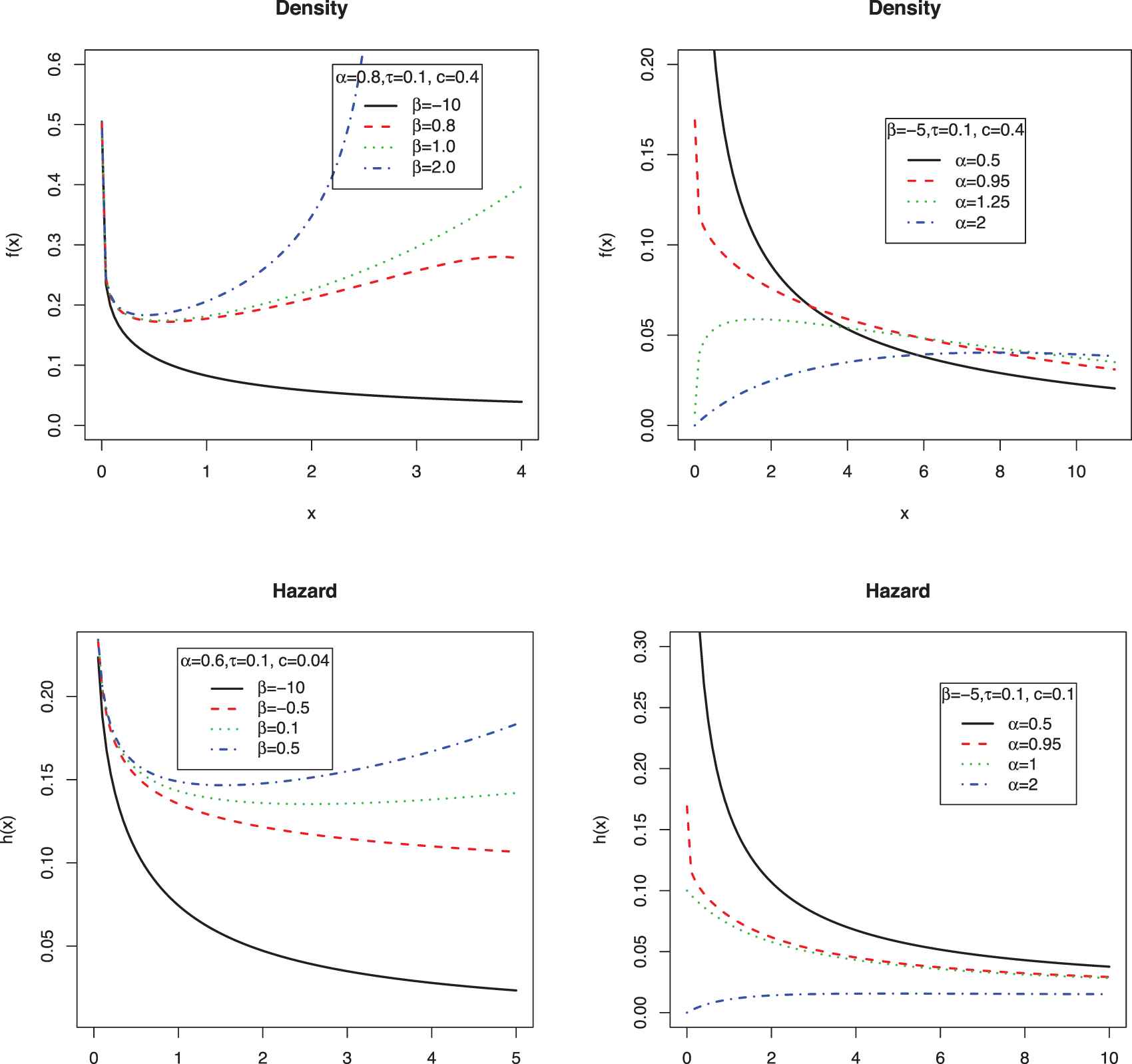
probability density function (pdf) and hazard rate function (hrf) of extended generalized Gompertz (EGG) distribution.
The limiting behaviors of pdf and hrf of the EGG distribution are as follows:
3. PROPERTIES
In this section, some measure such as the quantile function, non-central moment and entropy measure for EGG distribution are obtained and discussed.
3.1. Quantiles
The quantile function of EGG distribution is
3.2. Moments and Characterization
Here, first, we obtain a theorem to compute the noncentral moment,
Theorem 3.1.
For
Proof.
The proof is done by using binomial series expansion and following formula resulted from [30], Section 2.321, as
Theorem 3.2.
All moments of
Proof.
See the Appendix.
Using Theorem 3.2, the moments of the EEG distribution exist when
| −1 | −1.5 | −2 | −4 | −4.5 | −5 | ||
|---|---|---|---|---|---|---|---|
| 2 | 1 | 0.595 | 0.750 | 0.922 | 1.703 | 1.913 | 2.127 |
| 2 | 0.512 | 0.875 | 1.384 | 5.037 | 6.376 | 7.891 | |
| 3 | 0.582 | 1.406 | 2.922 | 21.186 | 30.189 | 41.537 | |
| 4 | 0.829 | 2.906 | 7.998 | 115.83 | 185.72 | 283.98 | |
| 5 | 1.429 | 7.383 | 27.012 | 781.781 | 1410.264 | 2396.170 | |
| 0.5 | 1 | 0.253 | 0.307 | 0.366 | 0.641 | 0.717 | 0.794 |
| 2 | 0.165 | 0.272 | 0.421 | 1.493 | 1.887 | 2.335 | |
| 3 | 0.165 | 0.389 | 0.799 | 5.732 | 8.166 | 11.237 | |
| 4 | 0.221 | 0.763 | 2.087 | 30.085 | 48.238 | 73.767 | |
| 5 | 0.369 | 1.891 | 6.896 | 199.151 | 359.255 | 610.443 | |
Computation of
Remark 3.1
Consider
3.3. Entropy
In this part, for measuring the uncertainty amount of the
If
3.4. Ordered Statistics
In this section, the cdf and noncentral moments of ordered statistics from the EGG distribution are provided. Let
Theorem 3.3.
For
4. ESTIMATION
In this section, we discuss the maximum likelihood method to estimate the parameters of the EGG model based on a random sample of size
Unfortunately, the close form solution for the maximum likelihood estimation (MLE) of parameters does not exist, but one can provide them. As we see, when
As we know
To determine the asymptotic distribution of the MLEs of
Theorem 4.1.
Given
The asymptotic distribution of
5. MODELING A REAL DATA SET
The following data set has been provided by [34] and also analyzed by [23]. It represents the lifetimes of 50 devices.
To find the best model for above data, we compare EGG, EGE, GG, and GE distributions as competing models. For each model, we obtain the MLEs of parameters. Then, we calculate some statistics that are useful in detecting the fitting effect of above proposed distributions. These statistics as well as their p-values are famous in all fitting distribution problems. In Table 3, we provide these statistics. From the p-value of Kolmogorov-Smirnov (K-S) statistic, we find that all proposed distributions can be fitted to this data set. Also in Table 3, we provide some statistics such as Akaike information criterion (AIC), Corrected Akaike’s Information Criterion (AICC), and Bayesian information criterion (BIC) to find the best fit between all proposed distributions. The lowest values of AIC, AICC, and BIC are related to EGG model. Also, all p-values of likelihood ratio test (LRT) statistic are less than
| Distribution |
||||
|---|---|---|---|---|
| Statistic | EGG | EGE | GG | GE |
| 0.3098 | 0.5368 | 0.2624 | 0.7798 | |
| 5.0000 | 1.8199 | — | — | |
| 0.0010 | 0.0064 | 0.0001 | 0.0187 | |
| 0.0173 | — | 0.0828 | — | |
| 173.69 | 189.1973 | 222.2441 | 239.9951 | |
| K-S | 0.1371 | 0.1558 | 0.1146 | 0.2042 |
| p-value (K-S) | 0.3041 | 0.1763 | 0.5273 | 0.0309 |
| AIC | 355.3747 | 384.3945 | 454.2548 | 483.9903 |
| AICC | 356.2636 | 384.9163 | 454.7765 | 484.2456 |
| BIC | 363.0228 | 390.1306 | 459.9908 | 487.8143 |
| LRT | — | 31.0198 | 100.8801 | 132.6156 |
| p-value (LRT) | — | 0.0000 | 0.0000 | 0.0000 |
EGG, extended generalized Gompertz; EGE, extended generalized exponential; GG, generalized Gompertz; GE, generalized exponential; LRT, likelihood ratio test; K-S, Kolmogorov-Smirnov.
Fit criteria based on EGG, EGE, GG, and GE distributions.
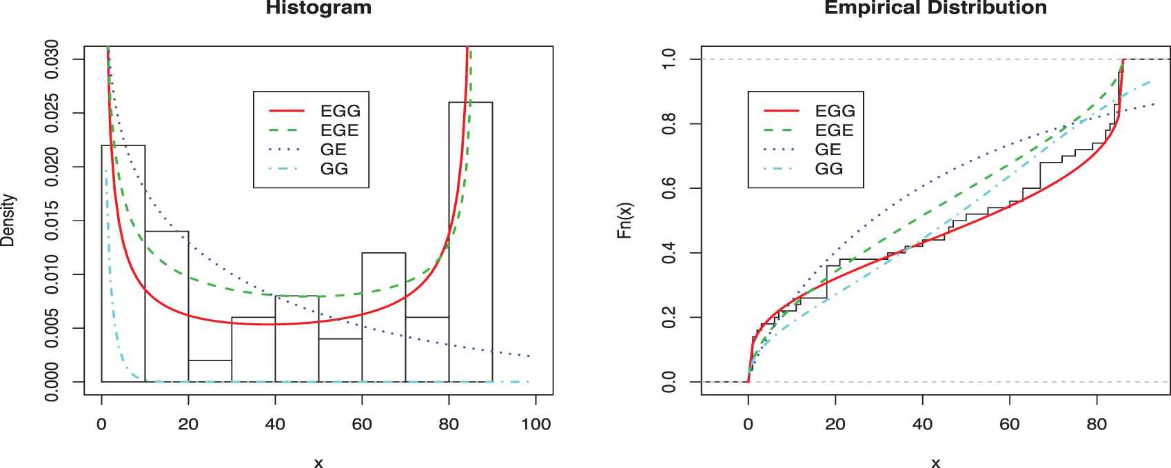
Fitting extended generalized Gompertz (EGG), extended generalized exponential (EGE), generalized Gompertz (GG), and generalized exponential (GE) distributions to the histogram (left) and the empirical cumulative distribution function (cdf) of the data (right).
CONFLICTS OF INTEREST
The authors declare that there are no conflicts of interest regarding the publication of this paper.
AUTHORS' CONTRIBUTIONS
All authors have read and agreed to the published version of the manuscript.
Funding Statement
There is no funding of this paper.
ACKNOWLEDGMENTS
The authors would like to thank the Editor in Chief of JSTA and the anonymous referees for many helpful comments and suggestions.
APPENDIX
A. Proof of Theorem 3.2
Let
whereSince
then using part (i), we can conclude thatSince
REFERENCES
Cite this article
TY  - JOUR
AU  - Mohammad Reza Kazemi
AU  - Ali Akbar Jafari
AU  - Saeid Tahmasebi
PY  - 2020
DA  - 2020/12/01
TI  - A Modification of the Gompertz Distribution Based on the Class of Extended-Weibull Distributions
JO  - Journal of Statistical Theory and Applications
SP  - 472
EP  - 480
VL  - 19
IS  - 4
SN  - 2214-1766
UR  - https://doi.org/10.2991/jsta.d.201116.001
DO  - 10.2991/jsta.d.201116.001
ID  - Kazemi2020
ER  -