Journal of Statistical Theory and Applications

Volume 19, Issue 2, June 2020, Pages 274 - 285

The Exponentiated Poisson-Exponential Distribution: A Distribution with Increasing, Decreasing and Bathtub Failure Rate

Authors
Francisco Louzada1, *, Vicente G. Cancho1, Paulo H. Ferreira2
1ICMC, Universidade de São Paulo São Carlos, São Paulo, Brazil
2DEst, Universidade Federal da Bahia Salvador, Bahia, Brazil
*Corresponding author. Email: louzada@icmc.usp.br
Corresponding Author
Francisco Louzada
Received 26 March 2019, Accepted 25 April 2020, Available Online 15 June 2020.
DOI
10.2991/jsta.d.200512.002How to use a DOI?
Keywords
Complementary risks; Exponentiated distributions; Maximum likelihood estimation; Poisson-Exponential distribution; Reliability and survival analysis
Abstract

In this paper we propose a new three-parameters lifetime distribution with increasing, decreasing and bathtub failure rate depending on its parameters. The properties of the proposed distribution are discussed, including explicit algebraic formulae for its reliability and failure rate functions, quantiles and moments. A simulation study is performed in order to verify the behavior of the maximum likelihood estimates. The methodology is illustrated on a real data set.

Copyright
© 2020 The Authors. Published by Atlantis Press SARL.
Open Access
This is an open access article distributed under the CC BY-NC 4.0 license (http://creativecommons.org/licenses/by-nc/4.0/).

1. INTRODUCTION

The exponential distribution (ED) provides an elegant, simple and close form solution to many problems in lifetime testing and reliability studies. However, the ED does not provide a reasonable parametric fit for some practical applications where the underlying failure rates are nonconstant, presenting monotone shapes. In recent years, in order to overcome such problem, new classes of models were introduced based on variations of the ED. For instance, Gupta and Kundu [1] proposed a generalized ED, which can accommodate data with increasing and decreasing failure rate function. Kus [2] proposed another modification of the ED with decreasing failure rate function, while Barreto-Souza and Cribari-Neto [3] generalizes the distribution proposed by [2] by including a power parameter in his distribution.

Recently, Cancho et al. [4] introduced the Poisson-Exponential (PE) distribution whose cumulative distribution function is given by

FPE(y;θ,λ)=eθeλyeθ1eθ,y>0,(1)
where θ>0 and λ>0. This distribution family based on the ED has increasing failure rate function.

As described by Marshall and Olkin [5], an exponentiated distribution can be easily constructed. It is based on the observation that by raising any baseline cumulative distribution function (cdf) Fbaseline(y) to an arbitrary power α>0, a new cdf F(y)=[Fbaseline(y)]α>0 is obtained, but now with the additional parameter α, which can be refereed as a resilience parameter and F(y) is a resilience parameter family. Although it is not our case, the term resilience easily emerges if we let θ be an integer. In this case, F(y) can be seem as the cdf of a parallel system with α independent components, which is less likely to failure as the number of components increases, leading to a resilient structure. Following this idea, several authors have considered extensions from usual survival distributions. For instance, Mudholkar et al. [6] considered the exponentiated Weibull distribution as a generalization of the Weibull distribution, [1] introduced the exponentiated ED as a generalization of the usual ED, Nadarajah and Kotz [7] proposed exponentiated type distributions extending the Fréchet, Gamma, Gumbel and Weibull distributions and Ristic and Nadarajah [8] introduced the exponentiated exponential-Poisson distribution as a generalization of the exponential-Poisson distribution due to [2].

Hence, the cdf of the exponentiated PE (EPE) distribution is defined from (1) as

F(y;θ,λ,α)=eθeλyeθ1eθα,y>0,(2)
where θ>0,λ>0 and α>0.

The paper is organized as follows: In Section 2 we present the probability density function, survival function and hazard function of the new distribution, the EPE distribution, and present graphics of such functions for some parameters values. Some properties of the EPE distribution are also presented in Section 2. In Section 3 we present the inferential procedure for the model parameters. Section 4 contains the results of a Monte Carlo simulation on the finite sample behavior of maximum likelihood estimates. In Section 5 the methodology is illustrated on a real data set. Some final comments in Section 6 conclude the paper.

2. THE EPE DISTRIBUTION

The probability density function (pdf) of the EPE distribution corresponding to the cdf (2) is given by

f(y)=αθλeλyθeλyeθeλyeθα1(1eθ)α,y>0,(3)
where θ>0,λ>0 and α>0. When α=1 the model (3) reduces to the PE distribution proposed by [4], and when α=1 and letting θ0+ the model (3) reduces to the ED with parameter λ.

If u and v are real numbers with |u|>|v| and γ>0, we have the series representation

(uv)γ1=k=0(1)kΓ(γ)Γ(γk)k!vkuγk1.(4)

If γ is an integer, the sum in (4) stops at γ1. Hence now eθeλy>eθ, we expand (eθeλyeθ)α1 as in Eq. (4) and then the pdf in (3) can be reduced to

f(y)=Γ(α+1)(1eθ)αk=0(1)keθ(α+k+1)eλyΓ(αk)(k+1)!fPE(y;θ(k+1),λ),(5)
where fPE(y;θ(k+1),λ) is the pdf of a random variable with PE distribution with parameters θ(k+1) and λ. We then have the EPE pdf can be written as a linear combination of PE pdfs. Figure 1 (left panel) shows the pdf (3) for some values of parameters.

Figure 1

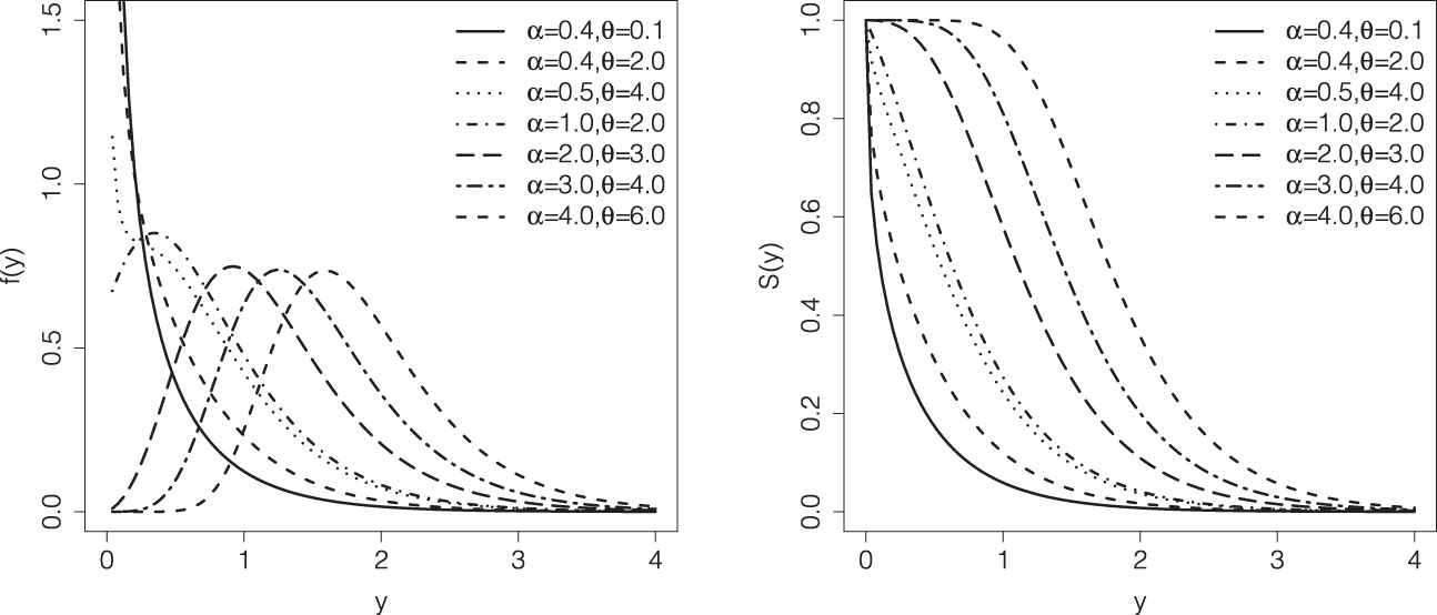
Left panel: probability density function of the exponentiated Poisson-Exponential (EPE) distribution. Right panel: survival function of the EPE distribution. We fixed λ = 2.

The EPE survival function is given by

S(y)=1eθeλyeθ1eθα,y>0.(6)

Figure 1 (right panel) shows some survival function shapes for same fixed values of θ and α.

The quantile q (yq, 0<q<1) of the EPE distribution is obtained by inverting Eq. (2) to give

yq=λ1log(θ)log(log(q1αeθ(q1α1))).

In particular, the median is y0.5=λ1log(θ)log(log(21αeθ(21α1))).

2.1. Failure Rate

From (3) and (6) it is easy to verify that the failure rate function is given by

h(y)=αθλeλyθeλyeθeλyeθα1(1eθ)α(eθeλyeθ)α,y>0.

The EPE distribution accommodates increasing, decreasing and bathtub failure rates depending on the parameter values. Define the function η(y)=f(y)f(y), where f(.) denotes the first derivative of f(.). Hence

η(y)=λθλeλy(α1)θλeλy1eθ(1eλy)1
and
η(y)=θλ2eλy1+(α1)1eθ(1eλy)(1θeλy)(1eθ(1eλy))2.

Considering the inequality

1eθ<1eθ(1eλy)(1θeλy)<θ
in equation above implies that if α1 then η(y)>0, y>0. Thus, from Glaser's theorem (see [9]), it follows that the failure rate function is increasing.

If θ1 and α<1 we have (α1)1eθw(1θ(1w))(1eθw)2<(1α)(1eθ)1<1, where w=1eλy, 0<w<1. It has η(y)<0. Hence, from Glaser [9], we conclude that the failure rate function is decreasing. We also observed that the failure rate function may be bathtub. The distinct types of failure rate shapes are illustrated in Figure 2 for some different parameter combinations of the EPE distribution.

Figure 2

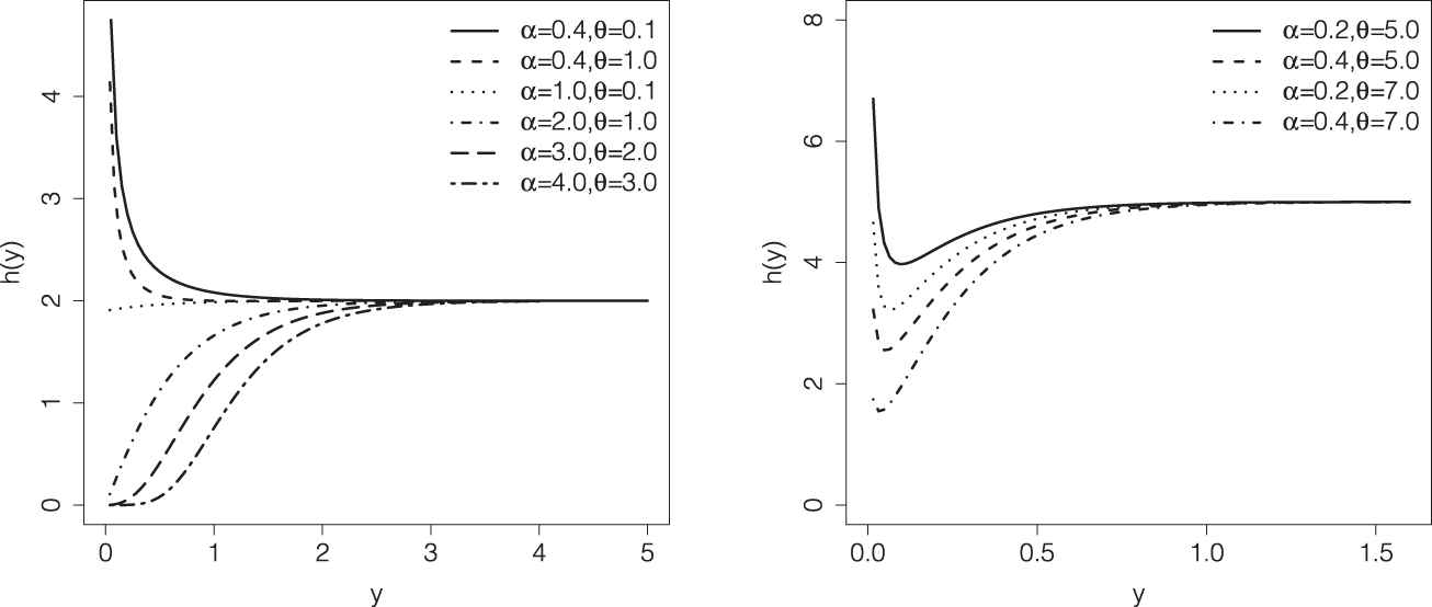
Failure rate function of the exponentiated Poisson-Exponential (EPE) distribution with λ = 2 (left panel) and λ = 5 (right panel) fixed.

2.2. Some Properties

Many of the most important features and characteristics of a distribution can be studied through its moments, such as mean, variance, tending, dispersion, skewness and kurtosis.

We shall now provide a general expression for the rth ordinary moment of the EPE distribution. Cancho et al. [4] showed that the rth moment of the random variable Y with PE distribution with parameters θ and λ can be expressed as

E[Yr]=θr!λr(1eθ)Fr+1,r+1([1,,1],[2,,2],θ),(7)
where
Fp,q(a,b,θ)=j=0θji=1pΓ(ai+j)Γ(ai)1Γ(j+1)i=1qΓ(bi+j)Γ(bi)1
is the generalized hypergeometric function, with a=[a1,,ap], p is the number of operands of a,b=[b1,,bq] and q is the number of operands of b.

We then formulate the following result.

Proposition 2.1.

Let Y be a random variable with EPE distribution and parameters θ, λ and α. If α>0 non-integer, using (5) and (7) we obtain the raw rth ordinary moment of Y can be written as

E[Yr]=θr!Γ(α+1)λr(1eθ)α+1k=0(1)keθ(α+k+1)eλyΓ(αk)(k+1)!Fr+1,r+1([1,,1],[2,,2],θ(k+1)),
where Fp,q(a,b,θ) is the generalized hypergeometric function.

Proof.

The proof is obtained by direct integration and it is then omitted.

Order statistics are among the most important tools in nonparametric statistics and inference. Let Y1,,Yn be a random sample taken from the EPE distribution and let Y1:n,,Yn:n denote the corresponding order statistics. The probability density function fi:n(y) of the ith order statistic Yi:n is given by

fi:ny=n!k1!nk!Fyk11Fynkfy.

According to Barakat and Abdelkader [10], the rth moment of the ith order statistic Yi:n can be represented as

EYi:nr=rp=ni+1n1pn+i1p1ninp0yr1Sypdy.(8)

Consider the binomial series expansion given by

1xr=k=0rkk!xk,(9)
where (r)k=r(r1)(rk+1) is a Pochhammer symbol. If |x|<1 the series converges and
rk=1krk+1k.(10)

We then state the following.

Proposition 2.2.

For the random variable Y with EPE distribution, we have that the rth moment of the ith order statistic is given by

EYi:nr=r!λrp=ni+1nk=0l=0m=01pn+i+kα+1+l+mp1ninp×pk+1kαkl+1lemlnθl+θαk+l1eθαkk!l!m!mr.

Proof.

From (6) and (8), and using (9), (10) and the Taylor series of the exponential function exi.eex=i=0xii!1i, we have that

EYi:nr=rp=ni+1n1pn+i1p1ninp0yr1Sypdy=rp=ni+1n1pn+i1p1ninp0yr11eθeλyeθ1eθαpdy=rp=ni+1nk=0(1)pn+i+k1p1ninppk+1k1eθαkk!×0yr1eθeλyeθαkdy=rp=ni+1nk=0(1)pn+i+k1p1ninppk+1k1eθαkeθαkk!×0yr1eθeλy11αkdy=rp=ni+1nk=0(1)pn+i+kα+11p1ninppk+1k1eθαkeθαkk!×0yr11eθeλy1αkdy=rp=ni+1nk=0l=0(1)pn+i+kα+1+l1p1ninp×pk+1kαkl+1l1eθαkeθαklk!l!0yr1eθleλydy=rp=ni+1nk=0l=0m=0(1)pn+i+kα+1+l+m1p1ninp×pk+1kαkl+1l1eθαkeθαklemlogθ+mloglΓrk!l!m!mλr=r!λrp=ni+1nk=0l=0m=0(1)pn+i+kα+1+l+m1p1ninp×pk+1kαkl+1lemlogθl+θαk+l1eθαkk!l!m!mr.

This completes the proof.

Given that a component survives up to time t0, i.e., there was no failure prior to time t, the residual life is the period beyond t until the time of failure and defined by the conditional random variable Yt|Y>t. In reliability, it is well-known that the mean residual life function and the ratio of two consecutive moments of residual life characterize the distribution uniquely (see [11]). Thus, we obtain the rth order moment of the residual life via the general formula

μrt=EYtr|Y>t=1Sttrytr1S(y)dy.(11)

Proposition 2.3.

For the random variable Y with EPE distribution, we have that the rth order moment of the residual life is given by

μrt=r!λr1eθeλteθ1eθαk=0l=0m=01kα+1+l+m×2kkαkl+1lemlogθltλ+θαk+l1eθαkk!l!m!mr,r1.

Proof.

From (11), using (6), (9), (10) and the Taylor series of the exponential function ex, and proceeding a similar way in the proof of Proposition 2.2 follow the result.

Then, we obtain the mean residual life of the EPE distribution as

μ1t=μt=1λ1eθeλteθ1eθαk=0l=0m=01kα+1+l+m×2kkαkl+1lemlogθltλ+θαk+l1eθαkk!l!m!m.

On the other hand, we analogously consider the reversed residual life and some of its properties. The reversed residual life can be defined as the conditional random variable tY|Yt, which indicates the time elapsed from the failure of a component given that its life is less than or equal to t. This random variable may also be called the inactivity time or time since failure (for more details, you may see [12] and [13]). Also, in reliability, the mean reversed residual life function and the ratio of two consecutive moments of reversed residual life determine the distribution uniquely.

The rth order moment of the reversed residual life can be obtained via the well-known formula

mrt=EtYr|Yt=1Ft0trtyr1F(y)dy.(12)

Proposition 2.4.

For the random variable Y with EPE distribution, we have that the rth order moment of the reversed residual life is given by

mrt=tλr21αλtr+1eθeλteθαk=0l=01k+lαk+1kellogθkλt2+θα+kk!l!lr2+1×rWhittakerMr2,r+12,lλt+WhittakerMr2+1,r+12,lλt,r1,
where WhittakerMμ,ν,z is the Whittaker M function, which can be defined in terms of the hypergeometric function as follows:
WhittakerMμ,ν,z=e12z12+νhypergeom12+νμ,1+2ν,z.

Proof.

From (12) and using Fy given by (2), we have that

1Ft0trtyr1F(y)dy=1eθeλteθ1eθα0trtyr1eθeλyeθ1eθαdy=reθeλteθα0ttyr1eθeλyeθαdy=reθαeθeλteθα0ttyr1eθeλy11αdy=r1αeθαeθeλteθα0ttyr11eθeλy1αdy.

Now using (9) and proceeding a similar way in the proofs of Propositions 2.2 and 2.3 follow the result.

Thus, the mean of the reversed residual life of the EPE distribution is given by

m1t=1α2t12λ32eθeλteθαk=0l=01k+lαk+1kellogθkλt2+θα+kk!l!l32×WhittakerM12,1,lλt+WhittakerM12,1,lλt.

The Bonferroni and Lorenz curves (see [14]) and Gini index have many applications not only in economics to study income and poverty, but also in other fields like reliability, insurance and medicine. The Bonferroni curve BF[F(y)] is given by

BFFy=1μFy0yufudu,(13)
or equivalently by
BF(p)=1μp0pF1tdt,
where p=F(y) and F1(t)=inf{y:F(y)t}.

Proposition 2.5.

From the relationship between the Bonferroni curve and the mean residual lifetime given by Theorem 2.1 of Pundir et al. [15], the Bonferroni curve of the distribution function F of EPE distribution is given by

BFFy=αθμλeθeλyeθαk=0l=01α+k+l1θk+1lαkkeθαk1k!l!l+12×1+λyl+11eλyl+1.

Proof.

From (13) and using fy given by (3) and Fy given by (2), we have that

1μFy0yufudu=1μeθeλyeθ1eθα0yuαθλeλuθeλueθeλueθα1(1eθ)αdu=αθλμeθeλyeθα0yueλuθeλueθeλueθα1du=αθλeθα1μeθeλyeθα0yueλuθeλueθeλu11α1du=αθλ1α1eθα1μeθeλyeθα0yueλuθeλu1eθeλu1α1du.

Now using (9) and making binomial expansion a similar way in the proofs of Propositions 2.22.4 follow the result.

Also, the Lorenz curve of F that follows the EPE distribution can be obtained via the expression LF[F(y)]=BF[F(y)]F(y).

The scaled total time and cumulative total time on test transform of a distribution function F are given by

SFFy=1μ0ySudu
and
CF=01SFFyf(y)dy,
respectively (see [15]). If F(y) is the EPE distribution function specified by (2), then using formula (9) and the Taylor series of the exponential function ex,
SFFy=1μλk=0l=0m=01k+l+m2kkαkl+1lθlm1emyλk!l!m!m1eθαkeθl
and
CF=αμλ1eθαk=0l=0m=0n=0o=0p=01α+k+l+m+n+o+p1×2kkαkl+1lαnn2ooθm+p+1lmn+1p1eλom+p+1k!l!m!n!o!p!m1eθαkeθα+l+n+1om+p+1.

Finally, the Gini index can be obtained from the relationship G=1CF.

3. INFERENCE

In this section we discuss inference and interval estimation for the model parameters.

3.1. Estimation by Maximum Likelihood

Let y=y1,,yn be a random sample of the EPE distribution with unknown parameter vector ϑ=θ,λ,α. The logarithm of likelihood function for ϑ is given by

(ϑ)=nlog(αθλ)λi=1nyiθi=1neλyinαlog(1eθ)+(α1)i=1nlog(eθeλyieθ).(14)

The maximum likelihood estimates (MLEs) of ϑ=θ,λ,α can be directly obtained by maximizing the log-likelihood function (14), or alternatively, by finding the solution for the following three nonlinear equations:

(ϑ)θ=nθnαeθ1i=1neλyi(α1)i=1neλyiθeλyieθeθeλyieθ=0,(15)
ϑλ=nλi=1nyi+θi=1nyieλyi+θα1i=1nyieλyiθeλyieθeλyieθ=0,(16)
ϑα=nα+i=1nlogeθeλyieθnlog1eθ=0.(17)

The Eq. (17) can be solved exactly for α, i.e.,

α̂=ni=1nlog1eθ̂eθ̂eλ̂yieθ̂1,
conditional upon the values of θ̂ and λ̂, where α̂,θ̂ and λ̂ are the MLEs for α,θ and λ, respectively. Therefore, it is sufficient to solve the Eqs. (15) and (16) iteratively in order to find the MLEs for θ and λ.

3.2. Interval Estimation

For EPE distribution the Fisher information matrix is given by

Iϑ=nI1ϑ=nıθ,θıθ,λıθ,αıθ,λıλ,λıλ,αıθ,αıλ,αıα,α,
where
ıθ,θ=1θ2+αeθ1eθ2α1Ee2λyeθ1eλy1eθ1eλy2Eeλyeθ1eλy1eθ1eλy,ıλ,λ=1λ2+θEy2eλy+θα1Ey2eλy1eθ1eλy+θEy2e2λyθ1eλy1eθ1eλy2,ıθ,λ=Eyeλyα1Eyeλy1θeλy1eθ1eλy+θEye2λye2λyθ1eλy1eθ1eλy2,ıα,α=α2,ıλ,α=θEyeλy1eθ1eλy,ıθ,α=1eθ1+Eeλyeθ1eλy1eθ1eλy.

The above expressions depend on some expectations that can be easily computed using numerical integration.

Large sample inference for the model parameters can be based, in principle, on the MLEs and their estimated standard errors. Following Cox and Hinkley [16], under suitable regularity conditions, it can be shown that

nϑ̂ϑDN30,I11ϑ,
as n. This asymptotic behavior remains valid if Fisher information is evaluated at the MLEs, ϑ̂, say I1ϑ̂. Alternative estimates can be obtained from the inverse observed information matrix I1ϑ̂ since it is a consistent estimator of I1ϑ. We can use the approximate trivariate normal N3ϑ,I1ϑ̂ distribution of ϑ̂ to construct approximate confidence regions for some parameters and survival function of EPE model.

For testing goodness of fit of the EPE distribution and for comparing this distribution with some of its special cases, we consider the likelihood ratio statistics (LRS). For instance, for comparing the EPE distribution with the PE distribution proposed by [4] for a given data set we consider the hypothesis test given by H0:α=1 versus H1:α1. In this case, the LRS is given by Λ=2θ̂,λ̂,α̂θ̃,λ̃,1, where θ̂,λ̂ and α̂ are the MLEs without restriction and θ̃ and λ̃ are the estimates under H0. Following [16], under H0 we assume an asymptotic chi-square distribution with one degree of freedom for Λ.

4. SIMULATION STUDY

This section presents the results of a simulation study that has been performed in order to verify the behavior of the standard errors, bias and root mean squared errors of the maximum likelihood estimators of θ,λ and α. We generated 1,000 samples of size n=30, 50, 100, 200 and 500 from the EPE distribution for each one of the three sets of values of ϑ=(θ,λ,α): 0.5,2.0,0.5, which corresponds to a decreasing failure rate function; 0.5,2.0,2.0, from which follows that the failure rate is increasing; and 2.0,2.0,0.5, whose failure rate function has a bathtub shape. The results are condensate in Table 1, which shows the averages of the 1,000 MLEs, Avϑ̂, together with their standard errors, SEϑ̂, bias, Bϑ̂, and root mean squared errors, RMSEϑ̂. Besides, Table 1 shows the coverage probability of the 95% confidence intervals for parameters of the EPE distribution, CPϑ. Table 1 indicates the following results: convergence has been achieved in all cases, i.e., for all three sets of parameter values; the biases are always smaller than one empirical SE. These results suggest the MLEs have performed consistently. The standard errors of the MLEs decrease when sample size increases. The empirical coverage probabilities are close to the nominal coverage level, 0.95. In particular, as sample size increases.

n ϑ Av(ϑ̂) SE(ϑ̂) B(ϑ^) RMSE(ϑ^) CP(ϑ)
(0.5,2.0,0.5) (1.222,2.422,0.498) (1.507,0.816,0.147) (0.722,0.422,0.002) (1.670,0.918,0.147) (0.993,0.950,0.951)
30 (0.5,2.0,2.0) (1.383,2.159,1.976) (2.087,0.444,0.863) (0.883,0.159,0.024) (2.265,0.472,0.863) (0.998,0.971,0.952)
(2.0,2.0,0.5) (2.484,2.141,0.535) (2.578,0.610,0.217) (0.484,0.141,0.035) (2.622,0.626,0.220) (0.995,0.948,0.945)
(0.5,2.0,0.5) (0.946,2.223,0.491) (1.167,0.635,0.115) (0.446,0.223,0.009) (1.248,0.672,0.115) (0.983,0.953,0.941)
50 (0.5,2.0,2.0) (1.181,2.110,1.937) (1.761,0.367,0.697) (0.681,0.110,0.063) (1.888,0.383,0.700) (1.000,0.964,0.971)
(2.0,2.0,0.5) (2.089,2.034,0.533) (1.745,0.468,0.166) (0.089,0.034,0.033) (1.746,0.469,0.169) (0.995,0.958,0.963)
(0.5,2.0,0.5) (0.812,2.163,0.489) (0.863,0.468,0.085) (0.312,0.163,0.011) (0.918,0.495,0.085) (0.974,0.948,0.950)
100 (0.5,2.0,2.0) (0.942,2.067,1.936) (1.244,0.262,0.555) (0.442,0.066,0.064) (1.320,0.270,0.559) (0.999,0.961,0.964)
(2.0,2.0,0.5) (2.037,2.007,0.513) (1.223,0.366,0.120) (0.037,0.007,0.013) (1.223,0.366,0.121) (0.990,0.943,0.943)
(0.5,2.0,0.5) (0.630,2.056,0.494) (0.636,0.351,0.070) (0.130,0.056,0.006) (0.649,0.355,0.070) (0.969,0.958,0.954)
200 (0.5,2.0,2.0) (0.741,2.037,1.962) (0.872,0.188,0.415) (0.241,0.037,0.038) (0.904,0.192,0.417) (1.000,0.965,0.974)
(2.0,2.0,0.5) (1.960,1.995,0.512) (0.873,0.248,0.080) (0.040,0.005,0.012) (0.874,0.248,0.081) (0.953,0.954,0.953)
(0.5,2.0,0.5) (0.538,1.985,0.490) (0.428,0.331,0.075) (0.038,0.015,0.010) (0.430,0.331,0.075) (0.956,0.949,0.951)
500 (0.5,2.0,2.0) (0.582,2.013,2.001) (0.572,0.125,0.287) (0.082,0.013,0.001) (0.578,0.125,0.287) (0.995,0.961,0.985)
(2.0,2.0,0.5) (2.014,1.997,0.500) (0.535,0.185,0.053) (0.014,0.003,0.000) (0.535,0.185,0.053) (0.962,0.939,0.947)
Table 1

The averages of the 1,000 maximum likelihood estimates (MLEs), Avϑ̂, their standard errors, SEϑ̂, bias, Bϑ̂, root mean squared errors, RMSEϑ̂, and the coverage probabilities of the 95% confidence intervals for parameters of the exponentiated Poisson-Exponential (EPE) distribution, CP(ϑ). The parameter vector is given by ϑ=(θ,λ,α).

5. APPLICATION

In this section we consider a real data set of 520 failure times (10,000's of hours) of industrial devices. Initially, in order to identify the shape of a lifetime data failure rate function we shall consider a graphical method based on the TTT plot (see [17]). In its empirical version, the TTT plot is given by Grn=i=1rYi:n+nrYr:ni=1rYi:n, where r=1,,n and Yi:n denote the order statistics of the sample. It has been shown that the failure rate function is decreasing (increasing) if the TTT plot is convex (concave). Even though the TTT plot is only a sufficient condition, not a necessary one for indicating the failure rate function shape, it is used here as a crude indicative of its shape. Figure 3 (upper-left panel) shows the TTT plot for the considered data, which is first convex and then concave. It indicates a bathtub-shaped failure rate function, which can be properly accommodated by a EPE distribution.

Figure 3

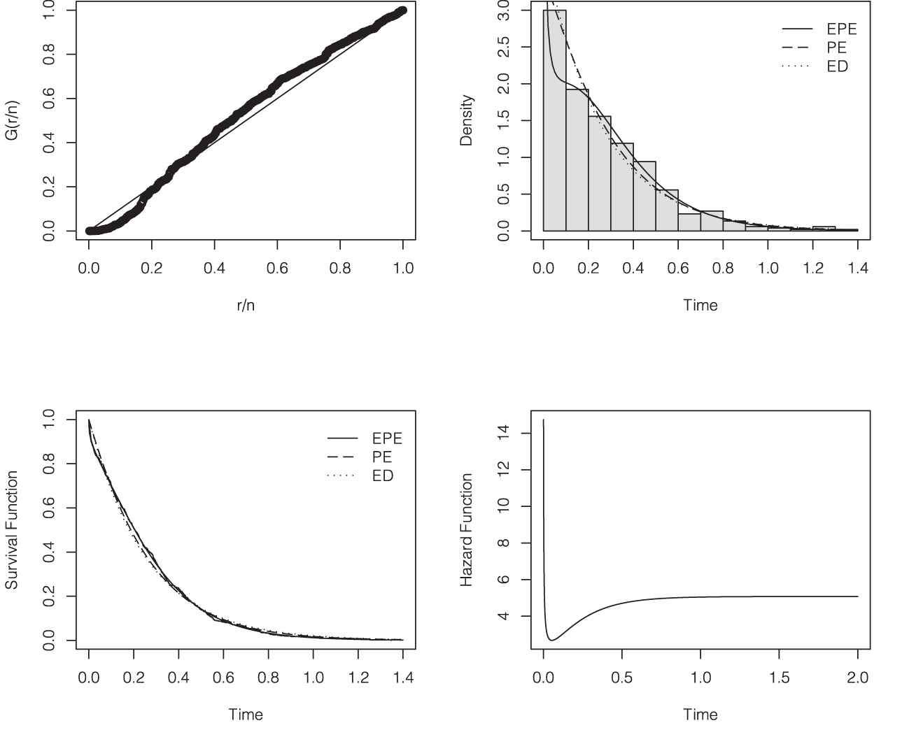
Upper-left panel: empirical scaled TTT-Transform on the real data set. Upper-right panel: histogram with estimated densities of the exponentiated Poisson-Exponential (EPE) distribution, PE distribution and exponential distribution (ED). Lower-left panel: Kaplan–Meier curve with estimated survival functions of the EPE distribution, PE distribution and ED. Lower-right panel: estimated hazard function of the EPE distribution.

Then, the EPE distribution was fitted to the data. Table 2 presents the MLEs and the corresponding 95% confidence intervals of the EPE distribution parameters, which were based on the Fisher information matrix at the MLEs, given by

I(ϑ^)=12.07710.895196.07310.89527.168149.504196.073149.5043736.717.

Parameter
Distribution θ λ α (.)
EPE 5.167 5.075 0.373 239.2338
[3.480; 6.854] [4.585; 5.565] [0.286; 0.460]
PE 0.362 4.204 183.1281
[0.086; 1.516] [3.606; 4.801]
ED 3.859 182.2578
[3.528; 4.191]

MLE, maximum likelihood estimate; EPE, exponentiated Poisson-Exponential; ED, exponential distribution; PE, Poisson-Exponential.

Table 2

MLEs and their corresponding 95% confidence intervals.

As discussed in Section 3.2, for comparison of nested models, which is the case when comparing the EPE distribution with the PE distribution and the PE distribution with the ED, we can compute the maximum values of the unrestricted and restricted log-likelihoods to obtain the LRS. Thus, the LRS used for testing H0:α=1 results in Λ=112.211 with p-value <0.0001, indicating that the EPE model presents a much better fitting than the PE model to the data set under consideration. The LRS used for testing H0:θ=0 (for details on this comparison, see results in [4]) is Λ=1.741 with p-value =0.187, which gives favorable evidence to the restricted model, i.e., the ED, over the full model, i.e., the PE model. The last column of Table 2 presents the log-likelihood values for the three fitted models. We also compare the EPE distribution, PE distribution and ED by inspection of the Akaike's information criterion (AIC), 2ϑ^+2k, and Schwarz's Bayesian information criterion (BIC), 2ϑ^+klog(n), where k is the number of parameters in the model and n is the sample size. The favorite model is the one with the smaller value on each criterion. The estimated statistics AIC and BIC for the EPE distribution are equal to 472.468 and 459.706, respectively. While, the estimated statistics AIC and BIC for the PE distribution are equal to 362.256 and 353.749, respectively; and the estimated statistics AIC and BIC for the ED are equal to 362.516 and 358.262, respectively. The EPE distribution overcomes the corresponding PE distribution and ED in both considered criterion. These results are corroborated by the plot in the lower-left panel of Figure 3, which compares the estimated survival functions obtained via ED, PE and EPE model fitting on the empirical Kaplan–Meier survival function. Figure 3 also shows the estimated densities (upper-right panel) and the hazard function obtained via EPE model fitting (lower-right panel).

Besides, for the sake of illustration, in order to compare our EPE distribution with other lifetime distributions capable of modeling a bathtub-shaped failure rate function, we fitted the exponentiated Nadarajah-Haghighi (ENH) distribution developed by Lemonte [18], with pdf given by

f(y)=αβλ(1+λy)α1exp{1(1+λy)α}[1exp{1(1+λy)α}]1β,y>0,
with all parameters α,β,λ>0. The MLEs of the parameters of the ENH model are given by α^=6.847,β^=0.606 and λ^=0.269, with the maximum log-likelihood value equal to ()=223.036. The estimated statistics AIC and BIC for the ENH distribution are equal to 440.071 and 427.310. Notice that our EPE distribution outperforms the ENH distribution in both considered criterion.

6. CONCLUDING REMARKS

In this paper we propose a new lifetime distribution. The EPE distribution is a generalization of the PE distribution proposed by [4], which accommodates increasing, decreasing and bathtub failure rate functions. It arises on a latent complementary competing risks scenario, where the lifetime associated with a particular risk is not observable but only the maximum lifetime value among all risks. We provide a mathematical treatment of this new distribution including explicit algebraic formulaes for its survival function and failure rate function, quantiles and moments. We discussed maximum likelihood estimation, which presented an adequate numerical stability in the simulation study performed. The EPE distribution allows a straightforwardly nested hypothesis testing procedure for comparison with its PE distribution particular case. The practical relevance and applicability of the EPE distribution were demonstrated in a real data set.

CONFLICT OF INTEREST

No conflict of interest has been reported by authors.

AUTHORS' CONTRIBUTIONS

(i) Vicente G. Cancho wrote the initial drafts of the paper and R codes; (ii) Paulo H. Ferreira helped in writing and improving the manuscript and the R programs, and also did the simulation study and analysis; and (iii) Francisco Louzada helped in the paper writing and supervised overall work.

ACKNOWLEDGMENTS

The research of Francisco Louzada is funded by the Brazilian organization CNPq.

REFERENCES

14.C.E. Bonferroni, Elementi di Statistica Generale, Seeber, Firenze, Italy, 1930.
Journal
Journal of Statistical Theory and Applications
Volume-Issue
19 - 2
Pages
274 - 285
Publication Date
2020/06/15
ISSN (Online)
2214-1766
ISSN (Print)
1538-7887
DOI
10.2991/jsta.d.200512.002How to use a DOI?
Copyright
© 2020 The Authors. Published by Atlantis Press SARL.
Open Access
This is an open access article distributed under the CC BY-NC 4.0 license (http://creativecommons.org/licenses/by-nc/4.0/).

Cite this article

TY  - JOUR
AU  - Francisco Louzada
AU  - Vicente G. Cancho
AU  - Paulo H. Ferreira
PY  - 2020
DA  - 2020/06/15
TI  - The Exponentiated Poisson-Exponential Distribution: A Distribution with Increasing, Decreasing and Bathtub Failure Rate
JO  - Journal of Statistical Theory and Applications
SP  - 274
EP  - 285
VL  - 19
IS  - 2
SN  - 2214-1766
UR  - https://doi.org/10.2991/jsta.d.200512.002
DO  - 10.2991/jsta.d.200512.002
ID  - Louzada2020
ER  -