Properties of Shannon Entropy for Double Truncated Random Variables and its Applications

Rajesh Moharana; Suchandan Kayal

doi:10.2991/jsta.d.200512.003

<Previous Article In Issue

Download article (PDF)

Next Article In Issue>

Volume 19, Issue 2, June 2020, Pages 261 - 273

Properties of Shannon Entropy for Double Truncated Random Variables and its Applications

Authors

Rajesh Moharana, Suchandan Kayal^*

Department of Mathematics, National Institute of Technology Rourkela, Rourkela-769 008, Odisha, India

^*Corresponding author. Email: suchandan.kayal@gmail.com

Corresponding Author

Suchandan Kayal

Received 4 January 2017, Accepted 20 December 2018, Available Online 8 June 2020.

DOI: 10.2991/jsta.d.200512.003 How to use a DOI?
Keywords: Shannon entropy; Generalized failure rate function; Generalized conditional mean; Stochastic ordering; Doubly truncated entropy ordering; Aging classes
Abstract: Doubly truncated data are sometimes encountered in several applications, mainly in survival and astronomical data analysis. This occurs when the data falls between two points. In this study, we focus on the Shannon entropy measure of doubly truncated random variables. We propose ordering and various aging properties based on this measure. Characterizations of some useful life distributions are obtained. It is showed that under certain condition, the proposed measure determines the distribution function uniquely. Some results on discrete distributions are presented. Finally, applications are given.
Copyright: © 2020 The Authors. Published by Atlantis Press SARL.
Open Access: This is an open access article distributed under the CC BY-NC 4.0 license (http://creativecommons.org/licenses/by-nc/4.0/).

1. INTRODUCTION AND PRELIMINARY RESULTS

Analyzing uncertainty in truncated data have received wide attention from several authors in last two decades due to its relevance in various applied fields such as reliability theory, survival analysis, astronomy and economy. Double truncation of survival data occurs when event time of an individual lies within a certain interval. An individual is not observed if its event time does not lie in a pre-determined interval. In this case, the investigator has no information about this individual. There are several situations which lead to doubly truncated (interval) data. Few examples are given below.

In astronomy, due to resolution of telescopes, the luminosity of stars may be undetected if it is either too dim or too bright (see Efron and Petrosian [1]).
In survival analysis, generally one has information about the lifetime of a mechanical component/system in a particular time interval.
In biological science, the data of induction times in AIDS are doubly truncated since HIV was unknown before the year 1982. Thus infected patients would have been incorrectly discarded when developing AIDS before 1982 (see Bilker and Wang [2]).

For some applications of doubly truncated data in biomedical problems, we refer to Stovring and Wang [3], Zhu and Wang [4] and Moreira et al. [5]. In this paper, we consider Shannon differential entropy (see Shannon [6]) for the doubly truncated data. The Shannon entropy for doubly truncated random variable was proposed by Sunoj et al. [7]. Later, it was studied by Misagh and Yari [8]. Let X be a nonnegative random variable or random lifetime of a component with cumulative distribution function (cdf) F(x), survival function (sf) F¯(x) and probability density function (pdf) f(x). The hazard and reversed hazard rate functions of X are denoted by λF(x)=f(x)∕F¯(x) and ηF(x)=f(x)∕F(x), respectively. The pdf of the doubly truncated random variable X[t1,t2]=(X|t1<X<t2) is f(x)∕ΔF, where ΔF=F(t2)−F(t1) and 0<t1<x<t2<∞. X[t1,t2] can be thought of the time to failure of a system which fails in the interval (t1,t2), where (t1,t2)∈D={(x,y)|F(x)<F(y)}. The Shannon entropy of X[t1,t2] is given by

SX(t1,t2)=−∫t1t2f(x)ΔFlnf(x)ΔFdx.(1.1)

This is called the doubly truncated entropy. In particular, (1.1) reduces to the residual (left truncated) entropy when t2→∞, to the past (right truncated) entropy when t1→0, and to the usual differential entropy when t1→0 and t2→∞. The expression in (1.1) quantifies the expected uncertainty of the random lifetime X of a system given that the system has survived up to time t1 and has been found to be down at time t2. It plays a significant role in studying different characteristics of a reliability component which fails in a time interval. Further, there exist two distributions which do not have the same doubly truncated entropy though they have same entropy. This motivates us to study properties of the doubly truncated entropy given by (1.1). For some recent developments on information theoretic measures for doubly truncated random variables, we refer to Kundu [9,10].

Next, we recall few preliminary results which are useful in the rest of the paper. The failure rate function of a nonnegative random variable X with cdf F(x) and pdf f(x) can be generalized for doubly truncated random variable (see Navarro and Ruiz [11]). The generalized failure rate (GFR) functions of X are given as

h1(t1,t2)=f(t1)ΔFandh2(t1,t2)=f(t2)ΔF.(1.2)

Note that h1(t1,∞)=λF(t1) and h2(0,t2)=ηF(t2). Navarro and Ruiz [11] studied the GFR functions given by (1.2) in detail. Authors showed that they determine the distribution function uniquely. Below, we state few definitions from Shaked and Shanthikumar [12].

Definition 1.1

Let X and Y be two nonnegative random variables with cdfs F(x) and G(x), sfs F¯(x) and G¯(x), pdfs f(x) and g(x) and hazard rate functions λF(x) and λG(x), respectively. Then

X is said to be smaller than Y in usual stochastic ordering, denoted by X≤stY if F¯(x)≤G¯(x) for all x.
X is said to be smaller than Y in likelihood ratio ordering, denoted by X≤lrY if g(x)∕f(x) is increasing in the union of the supports of X and Y.

The paper is arranged as follows: In Section 2, we define a new uncertainty order for two doubly truncated distributions. We obtain sufficient conditions under which the proposed order holds. New aging classes of lifetime distributions based on the doubly truncated entropy are proposed and some associated results are obtained in Section 3. In Section 4, we provide characterizations of some useful continuous distributions based on (1.1) including its uniqueness property. In Section 5, we discuss the concept of discrete doubly truncated entropy and obtain characterization result. Further, based on the doubly truncated entropy, how to choose a better system is presented in Section 6. Some concluding remarks have been added in Section 7.

Throughout the paper, we assume that the terms increasing and decreasing are used in nonstrict sense. All expectations, differentiations and integrations whenever used are assumed to exist. The random variables are taken to be nonnegative.

2. ORDER BASED ON DOUBLY TRUNCATED ENTROPY

In Example 2.1, we notice that even though the Shannon entropy of two units with random lifetimes X and Y are same, their corresponding expected uncertainty contained in the conditional distribution of X given t1<X<t2 is not same to that contained in the conditional distribution of Y given t1<Y<t2. Motivated by this, in this section, we define order based on the Shannon entropy for doubly truncated random variable and study its properties.

Definition 2.1

Let X and Y be two nonnegative and absolutely continuous random variables with pdfs f(x),g(x) and cdfs F(x),G(x), respectively. Then X is said to be smaller (larger) than Y in doubly truncated entropy order, denoted by X≤DTE(≥DTE)Y, if SX(t1,t2)≤(≥)SY(t1,t2) for all 0<t1<t2<∞.

Note that in particular, if t2→∞(t1→0), doubly truncated entropy order defined above becomes residual (past) entropy order. See, for instance, Ebrahimi and Pellerey [13], Nanda and Paul [14] for some properties on the residual and past entropy orderings. The physical interpretation of X≤DTE(≥DTE)Y can be easily understood from Definition 2.1. Let SX(t1,t2) and SY(t1,t2) quantify the amount of uncertainties of two mechanical components/systems with lifetimes X and Y. Then X≤DTE(≥DTE)Y implies that the expected uncertainty contained in the conditional density of X given that t1<X<t2 about the predictability of the failure time of the first component is less (greater) than that of Y given that t1<Y<t2 about the predictability of the failure time of the second component.

In the following, we consider example to show that there exist distributions which satisfy doubly truncated entropy order. It also illustrates the importance of the doubly truncated entropy over the Shannon entropy.

Example 2.1

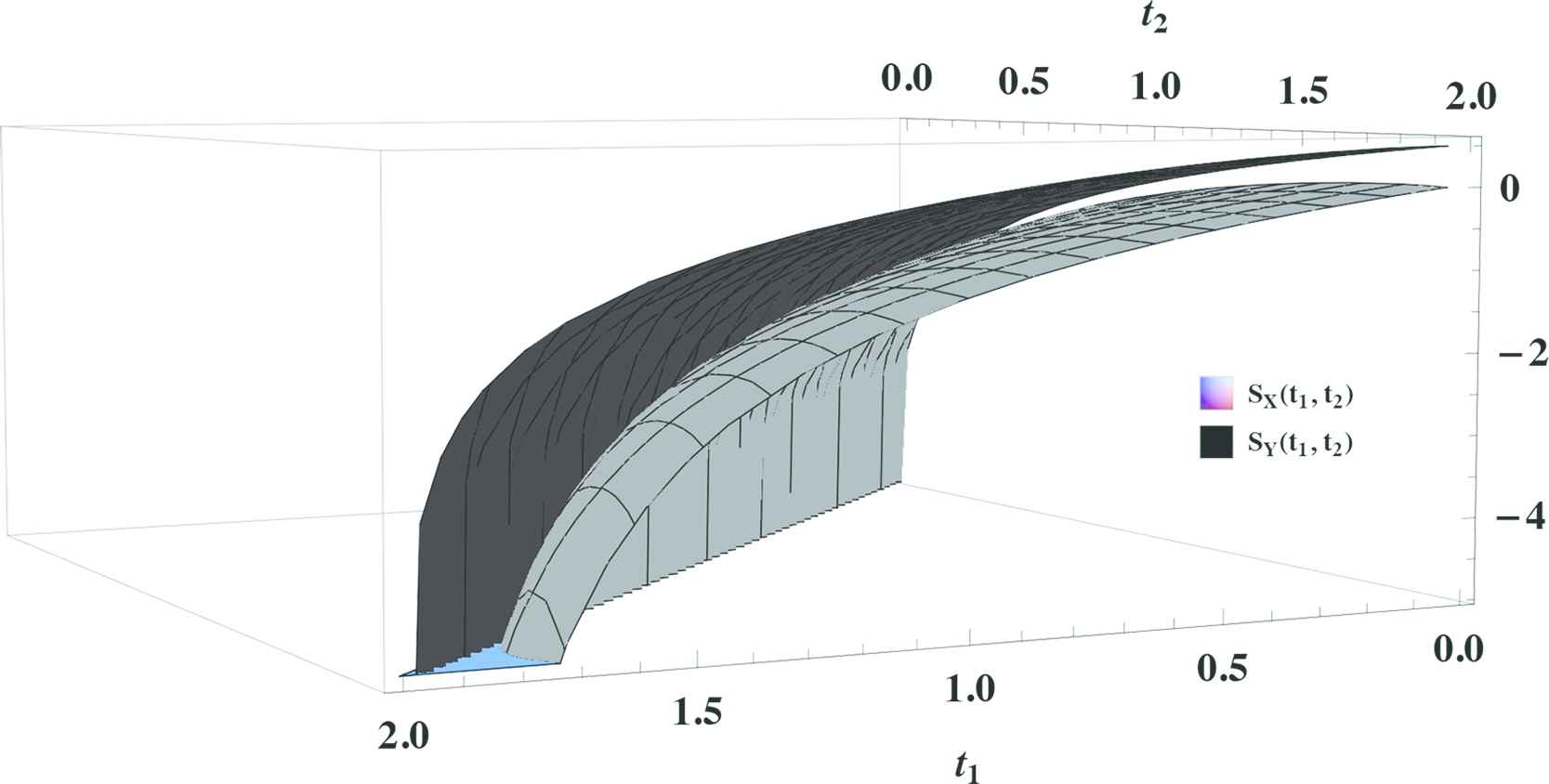
Let X and Y be two random variables with respective pdfs f(x)=(2−x)∕2 for x∈(0,2) and g(x)=x∕2 for x∈(0,2). One may easily show that SX=0.5=SY, that is, the Shannon entropies of the distributions corresponding to X and Y are equal. Further

SX(t1,t2)=−∫t1t22(2−x)(4t2−t22)−(4t1−t12)ln2(2−x)(4t2−t22)−(4t1−t12)dx(2.1)

and

SY(t1,t2)=−∫t1t22xt22−t12ln2xt22−t12dx.(2.2)

To compare SX(t1,t2) and SY(t1,t2), we plot (2.1) and (2.2) by Mathematica software, which are presented in Figure 1. The graphs of Figure 1 show that SX(t1,t2)≤SY(t1,t2) and hence X≤DTEY.

Stochastic orders have been a useful tool in many diverse areas of probability and statistics. In economics and finance, it plays an important role to obtain various bounds and inequalities. It is also used to compare different stochastic systems in reliability and life testing studies (see Shaked and Shanthikumar [12]). For the random variables X and Y considered in Example 2.1, it is easy to check that X≤lrY. Also, in this case X≤DTEY. Looking at this result, one may think about the possibility of the implication “X≤lrY⇒X≤DTEY.” But this implication does not hold in general, which is shown in the following counterexample. That is, the likelihood ratio order does not imply the doubly truncated entropy order in general. Mathematically,

X≤lrY⇏X≤DTEY.

Counterexample 2.1

Let X and Y be two random variables with cdfs F(x)=2x−x2 and G(x)=x2, respectively, where x∈(0,1). It is easy to check that X≤lrY. However, X≰DTEY, since SX(t1,t2)−SY(t1,t2)=0.040183(>0) at (t1=0.7,t2=0.9) and SX(t1,t2)−SY(t1,t2)=−0.065154(<0) at (t1=0.1,t2=0.6).

Thus, naturally the question arises: under which conditions likelihood ratio order follows doubly truncated entropy order? We find the answer of this question in the following theorem.

Theorem 2.1

Let X and Y be two nonnegative and absolutely continuous random variables having pdfs f(x) and g(x), respectively and X≤lr(≥lr)Y. Then

X≥DTEY if f(x) is increasing (decreasing) in x>0.
X≤DTEY if g(x) is decreasing (increasing) in x>0.

Proof.

Assume that X≤lr(≥lr)Y. Then making use of Theorem 1.C.5 of Shaked and Shanthikumar [12], we obtain [X|t1<X<t2]≤st(≥st)[Y|t1<Y<t2]. Moreover, from the assumption given by (i), we have f(x)∕ΔF is increasing (decreasing) function in x. Thus from (1.A.7) of Shaked and Shanthikumar [12], we obtain

Elnf(X)ΔF|t1<X<t2≤Elnf(Y)ΔF|t1<Y<t2.(2.3)

Further, the doubly truncated Kullback–Leibler measure (see Misagh and Yari [8]) can be written as

KLY,X(t1,t2)=∫t1t2g(x)ΔGlng(x)∕ΔGf(x)∕ΔFdx =−SY(t1,t2)−∫t1t2g(x)ΔGlnf(x)ΔFdx ≥0.(2.4)

The knowledge of (2.3) and (2.4) allows us to get SX(t1,t2)≥SY(t1,t2), which implies X≥DTEY. This completes the proof of the first part of theorem. The proof of the second part is similar to that of the first part, and is therefore omitted here for the sake of brevity.

In order to show the applicability of the above theorem we consider the following consecutive examples.

Example 2.2

Let X and Y be two random variables with pdfs f(x)=2x and g(x)=3x2, respectively, where x∈(0,1). It is easy to show that X≤lrY. Also, f(x) is increasing in x>0. Hence from Theorem 2.1, we have X≥DTEY.

Example 2.3

Let X and Y be two random variables following exponential distributions with pdfs f(x)=λ1exp{−λ1x} and g(x)=λ2exp{−λ2x}, respectively, for x>0 and λ1,λ2>0. For λ1>λ2, it is not hard to show that X≤lrY. Therefore, an application of Theorem 2.1 provides X≤DTEY, since the pdf of Y is decreasing in x>0.

Remark 2.1

From Theorem 1.C.5 of Shaked and Shanthikumar [12], we know that

X≤lrY⇔X[t1,t2]≤stY[t1,t2].

Thus the above results which are true for the likelihood ratio order, are also true for X[t1,t2]≤stY[t1,t2].

The following theorem shows that the doubly truncated entropy order is closed under increasing transformations.

Theorem 2.2

Let X and Y be two nonnegative and absolutely continuous random variables. Define ϕ(X)=aX+b and ϕ(Y)=aY+b, where a>0 and b≥0. Then for t1>b,

ϕ(X)≤DTE(≥DTE)ϕ(Y)ifX≤DTE(≥DTE)Y.

Proof.

For a nonnegative and absolutely continuous random variable X, under the given assumption and from Theorem 4.1 of Kundu [9], it can be shown that

Sϕ(X)(t1,t2)=SXt1−ba,t2−ba+lna.(2.5)

This observation completes the proof of the theorem.

3. NEW CLASS OF LIFETIME DISTRIBUTIONS BASED ON DOUBLY TRUNCATED ENTROPY

The classes of life distributions have various applications in reliability engineering, survival analysis and biological science. Based on some aspects of aging, life distributions can be classified. These classifications can be useful in modeling survival data. See, for instance, Barlow and Proschan [15], Zacks [16] and Lai and Xie [17]. These motivations and reasons lead theoreticians and reliability practitioners to propose nonparametric classes of distributions based on the notion of the Shannon entropy when random variables are truncated from left, as well as right. See for example, Ebrahimi and Pellerey [13], Ebrahimi [18], Ebrahimi and Kirmani [19] and Nanda and Paul [14]. In the present section, we propose a nonparametric class of distributions based on the doubly truncated Shannon entropy given by (1.1).

Definition 3.1

A nonnegative and absolutely continuous random variable X is said to be increasing doubly truncated entropy in t2, denoted by IDTE (t2), if and only if for any fixed t1, SX(t1,t2) is increasing in t2.

Remark 3.1

Following Nourbakhsh and Yari [20], another class based on the decreasing behavior of the doubly truncated Shannon entropy can be constructed. A nonnegative random variable X is said to be decreasing doubly truncated entropy in t1, denoted by DDTE (t1), if and only if for any fixed t2, SX(t1,t2) is decreasing in t1. Note that Nourbakhsh and Yari [20] proposed this class for doubly truncated generalized entropy. They have not studied this in detail. Below, we study this class with the class defined in Definition 3.1 in detail.

Remark 3.2

From (2.5), we note that the nonparametric classes described above are closed under increasing scale and location transformations.

There are many distributions which belong to these classes. For example, the uniform distribution belongs to IDTE (t2) class and the exponential distribution with mean λ>0 belongs to DDTE (t1) class. Indeed, both the distributions belong to both DDTE (t1) and IDTE (t2) class. The following counterexamples show that there exist distributions which are not monotone in terms of the doubly truncated entropy, in t1 for any fixed t2, and in t2 for any fixed t1.

Counterexample 3.1

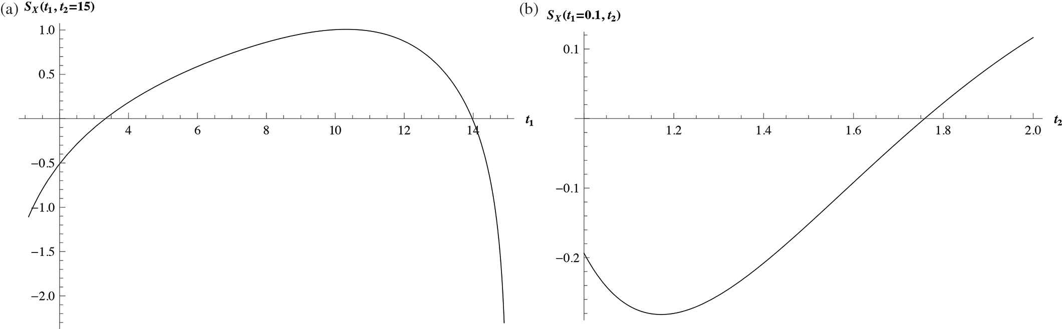
Let X be a random variable with distribution function F(x)=1−(a∕x)b,x>a,a>0,b>0. Consider a=1 and b=10. We plot the doubly truncated entropy for this distribution in Figure 2(a), which shows that the doubly truncated entropy is not monotone in t1 for some fixed t2.

Counterexample 3.2

Consider a nonnegative random variable with distribution function

F(x)=exp{−1∕2−1∕x},0≤x≤1,exp{−2+x2∕2},1≤x≤2.(3.1)

Figure 2(b) represents the graphical plot of SX(t1,t2) for the random variable with distribution function given by (3.1). It shows that SX(t1,t2) is not monotone in t2 for some fixed t1.

The following theorem shows that there exists no nonnegative random variable having increasing (decreasing) doubly truncated entropy in t1(t2) for any fixed t2(t1). That is, the classes IDTE (t1) and DDTE (t2) are empty.

Theorem 3.1

Let X be a nonnegative and absolutely continuous random variable with cdf F(x). Then

SX(t1,t2) can not be an increasing function in t1 for any fixed t2.
SX(t1,t2) can not be a decreasing function in t2 for any fixed t1.

Proof.

Using L-Hospital's rule, the proof follows along the similar arguments of that of Theorem 2.2 of Khorashadizadeh et al. [21].

Theorem 3.2

Let X be a nonnegative and absolutely continuous random variable. Define Z=aX+b, where a>0 and b≥0 are constants.

If X belongs to DDTE (t1), then Z belongs to DDTE (t1).
If X belongs to IDTE (t2), then Z belongs to IDTE (t2).

Proof.

From Definition 3.1 and (2.5), the proof follows.

The following example can be viewed as an application of Theorem 3.2.

Example 3.1

Let X be a random variable with pdf f(x|a,b,α,β)=α(x−β)2 for a<x<b, where α=12∕(b−a)3, β=(a+b)∕2, and −∞<a<b<∞. This is known as U-quadratic distribution which is useful in electronics and communication. For example, reference signals for a Stochastic Analog-to-Digital Converter can be generated by a simple resistor ladder which follows the U-quadratic distribution. Here, it is easy to show that X and cX+d, where c>0 and d≥0 belong to both DDTE (t1) class and IDTE (t2) class.

There are several situations where one may be interested to know whether DDTE (t1) and IDTE (t2) properties of a nonnegative random variable X are inherited by a transformation of X. The following consecutive theorems provide us partial answer to that.

Theorem 3.3

Let X be a nonnegative and absolutely continuous random variable belongs to DDTE (t1) class. If ϕ is a nonnegative, strictly increasing, concave function, then ϕ(X) also belongs to DDTE (t1) class.

Proof.

From Theorem 4.1 of Kundu [9] we have

SϕXt1,t2=SXϕ−1t1,ϕ−1t2+Elnϕ′X|ϕ−1t1<X<ϕ−1t2,(3.2)

where ϕ(x) is strictly increasing. Under the given assumptions, SX(ϕ−1(t1),ϕ−1(t2)) decreases with respect to t1 for fixed t2. The second term of the right hand side expression of (3.2) also decreases in t1. Combing these with (3.2), the theorem is proven.

Theorem 3.4

Let X be a nonnegative and absolutely continuous random variable belonging to IDTE (t2) class. If ϕ is a nonnegative, strictly increasing, convex function, then ϕ(X) also belongs to IDTE (t2) class.

Proof.

The proof is analogous to that of Theorem 3.3 and is therefore omitted here for the sake of brevity.

As an application of Theorems 3.3 and 3.4, we consider the following example.

Example 3.2

Let X be a random variable following exponential distribution with pdf f(x|λ)=λexp{−λx}, where x>0 and λ>0. It is easy to see that X belongs to both DDTE (t1) class and IDTE (t2) class. Consider the transformation Y=ϕ(X)=X1∕α,α>0, which is nonnegative, strictly increasing and convex (concave) function for 0<α<1(α>1). Moreover, ϕ(X) follows Weibull distribution with distribution function G(x)=1−exp{−λxα},x>0. Therefore, Theorems 3.3 and 3.4 yield that Weibull distribution also belongs to both DDTE (t1) class and IDTE (t2) class.

The following theorem provides upper bounds of SX(t1,t2) in terms of the GFR functions for the distributions belonging to the classes defined above. We omit the proof since the results can be easily obtained.

Theorem 3.5

Let X be a nonnegative and absolutely continuous random variable.

If X belongs to DDTE(t1) class, then SX(t1,t2)≤1−lnh1(t1,t2).
If X belongs to IDTE(t2) class, then SX(t1,t2)≤1−lnh2(t1,t2).

4. SOME CHARACTERIZATION RESULTS AND BOUNDS

Characterizations of statistical distributions are important concept in modeling statistical data as these are useful to describe the distribution. Because of this, several authors studied characterizations of various statistical distributions. For some characterization results based on left truncated (residual) and right truncated (past) entropies, we refer to Belzunce et al. [22] and Nanda and Paul [14]. In this section, we obtain some characterization results based on SX(t1,t2) given by (1.1). Misagh and Yari [8] showed that under some conditions, the doubly truncated entropy uniquely determines the distribution function. We obtain characterization based on the condition involving the concept of generalized conditional mean of X[t1,t2]. It is given by

μX(t1,t2)=∫t1t2xf(x)ΔFdx,(4.1)

which has been used in various contexts of reliability theory involving stochastic orders and characterizations of doubly truncated random lifetimes. The following lemma is useful to prove our next theorem.

Lemma 4.1

(Navarro and Ruiz [11]) GFR functions h1(t1,t2) and h2(t1,t2) of the random variable X determine the distribution function uniquely.

Theorem 4.1

Let X be a nonnegative and absolutely continuous random variable such that SX(t1,t2)=μX(t1,t2). Then SX(t1,t2) determines the distribution function uniquely.

Proof.

Differentiating (1.1) with respect to t1 (for any fixed t2) and t2 (for any fixed t1) we get

∂SX(t1,t2)∂t1=h1(t1,t2)[SX(t1,t2)+lnh1(t1,t2)−1]and(4.2)

∂SX(t1,t2)∂t2=−h2(t1,t2)[SX(t1,t2)+lnh2(t1,t2)−1],(4.3)

respectively. Further from (4.1), we have

∂μX(t1,t2)∂t1=h1(t1,t2)[μX(t1,t2)−t1]and(4.4)

∂μX(t1,t2)∂t2=−h2(t1,t2)[μX(t1,t2)−t2].(4.5)

Thus, from the given assumption and (4.2), (4.3), (4.4), (4.5), we obtain

lnh1(t1,t2)+t1−1=0and(4.6)

lnh2(t1,t2)+t2−1=0.(4.7)

Therefore, for any fixed t2 and arbitrary t1, h1(t1,t2) is a positive solution of the equation g1(x)=0, where g1(x)=lnx+t1−1 and for any fixed t1 and arbitrary t2, h2(t1,t2) is a positive solution of the equation g2(x)=0, where g2(x)=lnx+t2−1. Moreover, it is easy to show that both the equations g1(x)=0 and g2(x)=0 have unique positive solutions x=h1(t1,t2) and x=h2(t1,t2), respectively. Hence, using Lemma 4.1, the proof follows.

Next, we present a proposition for symmetric random variable. The proof is simple and thus omitted for brevity.

Proposition 4.1

Let X be a nonnegative, absolutely continuous and symmetric random variable with support [0,a], with finite a. Assume that it is symmetric with respect to a∕2. Then

SX(t1,t2)=SX(a−t2,a−t1).

As an application of Proposition 4.1, we consider the following example.

Example 4.1

Suppose X follows uniform distribution in (0,1). Here X is symmetric with respect to 1∕2. Then, SX(t1,t2)=SX(1−t2,1−t1)=ln(t2−t1).

Remark 4.1

From (4.4) and (4.5), it is not hard to see that ∂μX(t1,t2)∂t1≥0 and ∂μX(t1,t2)∂t2≥0, that is, the generalized conditional mean in (4.1) is increasing in t1 (for fixed t2) and in t2 (for fixed t1). Observing this, we remark that there exists a relevant difference between the generalized conditional mean and the doubly truncated Shannon entropy. From Counterexamples 3.1. and 3.2, we observe that the doubly truncated entropy is not necessarily increasing in t1 (for fixed t2) and in t2 (for fixed t1).

Hereafter, we provide characterizations for some useful lifetime distributions such as exponential, Pareto and finite range distributions. These distributions have prominant applications in real life problems. Exponential distribution is widely used in describing lifetimes of components, service times in queueing systems, time periods between two successive occurrences in a Poisson process. Pareto distribution has been an important model to investigate the city population, insurance risk and business failures. Finite range distributions are used to model data in reliability and life testing experiments and econometrics. First, we obtain the expressions of the doubly truncated entropy for these distributions in terms of the GFR functions, which are presented in Table 1.

Distribution	pdf	SX(t1,t2)
Exponential	f(x)=λexp{−λx},	1−lnλ+t1h1(t1,t2)−t2h2(t1,t2)+lnexp{−λt1}−exp{−λt2}.
	x>0,
	λ>0.
Pareto	f(x)=pq(1+px)q+1,	−ln(pq)+ln(1+pt1)−q+(1+pt2)−q+q+1q(1+pt1)h1(t1,t2)ln(1+pt1) −(1+pt2)h2(t1,t2)ln(1+pt2)+p.
	x>0,
	p,q>0.
Finite range	f(x)=αβ(1−αx)β−1,	−ln(αβ)+ln(1−αt1)β−(1−αt2)β+(1−β)αβ(1−αt1)h1(t1,t2)ln(1−αt1) −(1−αt2)h2(t1,t2)ln(1−αt2)+α.
	0<x<1∕α,
	β,α>0.

Table 1

Probability density functions and the expressions of SX(t1,t2).

Theorem 4.2

Let X be a nonnegative and absolutely continuous random variable with pdf f(x) and cdf F(x). Then the following relationship:

SX(t1,t2)=1b(1+at1)h1(t1,t2)(1−lnf(t1))−(1+at2)h2(t1,t2)(1−lnf(t2))+c +ln(F(t2)−F(t1)),(4.8)

where a,b and c are constants, holds if and only if X follows

exponential distribution with cdf F(x)=1−exp{−λx},x>0,λ>0 for c=0.
Pareto distribution with cdf F(x)=1−(1+px)−q,x>0,p>0,q>0 for c>0.
finite range distribution with cdf F(x)=1−(1−αx)β,0<x<1∕α,β>0,α>0 for c<0.

Proof.

Assume that the relation given in (4.8) holds. Then from (1.1) and (4.8), we obtain

b∫t1t2f(x)lnf(x)dx=(1+at1)f(t1)(lnf(t1)−1)−(1+at2)f(t2)(lnf(t2)−1)−c(F(t2)−F(t1)).(4.9)

After differentiating (4.9) with respect to ti,i=1,2, and simplifying we get

f′(ti)f(ti)=−b+c1+cti,(4.10)

which implies that the random variable X respectively follows exponential, Pareto and finite range distributions for c=0,c>0 and c<0. With the help of the Table 1, the converse part of the theorem can be verified by direct calculation. This completes the proof of the theorem.

Remark 4.2

It is remarked that the results in Theorem 3.5 of Nourbakhsh and Yari [20] do not reduce to the Theorem 4.2 when β tends to 1. Specifically, when β approaches to 1, the right-hand side expression of the Equation (5.4) of Nourbakhsh and Yari [20] is not equal to that of (4.8) of the present paper.

It is worth mentioning that the closed form expression of SX(t1,t2) for some lifetime distributions may not be available due to difficulty in the computation. For these cases, the bounds may be helpful to get some idea about the amount of uncertainty contained in the distribution. In the following, we obtain some bounds for SX(t1,t2).

Proposition 4.2

Let X be a nonnegative and absolutely continuous random variable. Then

SX(t1,t2)≥1−Ef(X)ΔF|t1<X<t2.(4.11)

≤t2−t1−1(4.12)

Proof.

The bounds given in (4.11) and (4.12) can be obtained from the well-known inequalities lnx≤x−1 and x−1≤xlnx, where x>0, respectively.

There is a wide class of distributions having monotone density functions. Next, we obtain bounds of the doubly truncated entropy for the distributions having monotone densities in terms of the GFR functions.

Proposition 4.3

Let X be a nonnegative and absolutely continuous random variable with cdf F(x) and pdf f(x). If f(x) is decreasing (increasing) in x, then

−lnh1(t1,t2)≤(≥)SX(t1,t2)≤(≥)−lnh2(t1,t2),(4.13)

where h1(t1,t2) and h2(t1,t2) are defined in (1.2).

Proof.

Let f(x) be decreasing (increasing) in x. Then for t1≤x≤t2, we have

f(t1)ΔF≥(≤)f(x)ΔF≥(≤)f(t2)ΔF.(4.14)

Thus from (4.14) and after some calculations, the required result follows.

Example 4.2

Consider a random variable which follows half logistic distribution with cdf F(x)=1−exp⁡{−x}1+exp⁡{−x} and pdf f(x)=2exp⁡{−x}(1+exp⁡{−x})2, where x>0. The GFR functions of X are given by

h1(t1,t2)=2exp⁡{−t1}(1+exp⁡{−t1})21−exp⁡{−t2}1+exp⁡{−t2}−1−exp⁡{−t1}1+exp⁡{−t1}(4.15)

and

h2(t1,t2)=2exp⁡{−t2}(1+exp⁡{−t2})21−exp⁡{−t2}1+exp⁡{−t2}−1−exp⁡{−t1}1+exp⁡{−t1}.(4.16)

Moreover, it is easy to verify that the density function f(x) is decreasing in x>0. Thus, as an application of Proposition 4.3, one can easily obtain the bounds of SX(t1,t2).

5. DISCRETE DOUBLY TRUNCATED RANDOM VARIABLE AND SOME CHARACTERIZATION RESULTS

Attention on the study of discrete failure data came relatively late in comparison to its continuous analogue. In recent past, several authors have given a considerable attention to study some information theoretic and reliability measures for left truncated, right truncated and doubly truncated random variables. See, for instance, Belzunce et al. [22], Nanda and Paul [14], Khorashadizadeh et al. [23], Kumar et al. [24] and Asha et al. [25]. In this section we obtain some characterization results for the Shannon entropy of discrete doubly truncated random variable.

Let X be a discrete random variable, which takes the values x1,x2,…,xl with probabilities p1,p2,…,pl, respectively, where l∈N. Here, N represents the set of natural numbers. Denote pl=P(X=xl) and P(l)=P(X≤xl) the probability mass function and distribution function of X, respectively. We denote P(X=l|i≤X≤j) the probability mass function of the doubly truncated random variable X with left truncation at xi and right truncation at xj, where i<j and i,j∈N. It is given by

P(X=l|i≤X≤j)=plP(j)−P(i−1),(5.1)

where 1≤i<l<j≤∞. Note that for i=1,(j=∞) (5.1) reduces to the probability mass function of the right (left) truncated discrete random variable. The GFR functions are given by (see Navarro and Ruiz [11])

hi(i,j)=piP(j)−P(i−1)(5.2)

and

hj(i,j)=pjP(j)−P(i−1).(5.3)

Then the discrete doubly truncated entropy is given by

S̃X(i,j)=−∑k=ijpkP(j)−P(i−1)lnpkP(j)−P(i−1).(5.4)

Note that when j=∞, then (5.4) becomes discrete residual entropy (see Belzunce et al. [22]) and when i=1, then it reduces to discrete past entropy (see Nanda and Paul [14]). They studied some characterization results for residual and past entropy of discrete random variables. The generalized conditional mean for the doubly truncated discrete random variable is given by

MX(i,j)=∑k=ijkpkP(j)−P(i−1).(5.5)

The following theorem shows that S̃X(i,j) determines the distribution function uniquely.

Theorem 5.1

Let X be a random variable with discrete distribution function P(t). If S̃X(i,j) is increasing in i (for fixed j) and decreasing in j (for fixed i), then S̃X(i,j) uniquely determines the distribution function.

Proof.

From (5.4) we have

∑k=ijpklnpk=(P(j)−P(i−1))ln(P(j)−P(i−1))−S̃X(i,j).(5.6)

Now replacing i by i+1 in (5.6) and then subtracting from (5.6), we obtain

pilnpi=[P(j)−P(i−1)]ln(P(j)−P(i−1))−S̃X(i,j) −[P(j)−P(i)]ln(P(j)−P(i))−S̃X(i+1,j).(5.7)

Further, replacing j by j+1 in (5.6) and then subtracting we get

pj+1lnpj+1=[P(j+1)−P(i−1)]ln(P(j+1)−P(i−1))−S̃X(i,j+1) −[P(j)−P(i−1)]ln(P(j)−P(i−1))+S̃X(i,j).(5.8)

Now consider fix j. Then substituting pi=[P(j)−P(i−1)]−[P(j)−P(i)] and λi=(P(j)−P(i))∕(P(j)−P(i−1)) in (5.7) and after some simplifications we get

g1(x)=(1−x)ln(1−x)+xlnx+S̃X(i,j)−xS̃X(i+1,j)=0,(5.9)

where x=λi,λi∈(0,1). Further, we take fix i. Then substituting pj+1=[P(j+1)−P(i−1)]−[P(j)−P(i−1)] and θj=(P(j)−P(i−1))∕(P(j+1)−P(i−1)) in (5.8) we obtain

g2(x)=(1−x)ln(1−x)+xlnx+S̃X(i,j+1)−xS̃X(i,j)=0,(5.10)

where x=θj,θj∈(0,1). Now we will show that for fixed j, g1(x)=0 in (5.9) has a unique positive solution x=λi for all i. It is easy to see that

g1(0)=S̃X(i,j)≥0andg1(1)=S̃X(i,j)−S̃X(i+1,j)≤0,(5.11)

and hence there exists at least one root of g1(x)=0 in (0,1). Now differentiating (5.9) with respect to x we get

g1′(x)=−S~X(i+1,j)+ln⁡(x1−x).(5.12)

Again, g1″(x)=1x(1−x), which is positive in (0,1). It implies that g1(x) is convex in (0,1). Thus using (5.11) we can say that for fixed j, g1(x)=0 has a unique positive solution in (0,1) for all i. Using similar arguments, it can be proved that for fixed i, g2(x)=0 has also a unique positive solution in (0,1) for all j. Further, 1−λi=hi(i,j) and 1−θj=hj+1(i,j+1), where hi(i,j) and hj+1(i,j+1) are discrete GFR functions of X. It is known that discrete GFR functions uniquely determine the distribution function (see Navarro and Ruiz [11]). Hence the proof is completed.

Remark 5.1

For j=∞, Theorem 5.1 reduces to Theorem 2 of Belzunce et al. [22].

Theorem 5.2

The discrete uniform distribution with support {1,2,…,n} is characterized by S̃X(i,j) decreasing in i (for fixed j) and increasing S̃X(i,j) in j (for fixed i) if and only if S̃X(i,j)=ln(j−i+1), where 1≤i<j≤n and i,j∈N.

Proof.

In case of discrete uniform distribution with support {1,2,…,n},

S̃X(i,j)=−∑k=ij1j−i+1ln1j−i+1 =ln(j−i+1).(5.13)

Further, suppose S̃X(i,j)=ln(j−i+1), for 1≤i≤j≤n and i,j∈N. Then from (5.9) g1(x)=0 has unique solution when g1(uj)=0. Now, using (5.12), we get that

uj=1+exp{−S̃(i+1,j)}−1=j−ij−i+1.

Thus, g1(x)=0 has unique solution given by x=uj. Moreover, λi is a solution of (5.9). Hence λi=(j−i)∕(j−i+1) is the unique solution of g1(x)=0. Again from (5.10), g2(x)=0 has a unique solution. Similar argument shows that θj=(j−i+1)∕(j−i+2) is the unique solution of g2(x)=0. Hence, the theorem is established.

Remark 5.2

Theorem 5.2 is a generalization of Remark 3 of Belzunce et al. [22] and Theorem 5.1 of Nanda and Paul [14]. The respective particular cases can be obtained by taking j=n and i=1.

Remark 5.3

In general, S̃X(i,j) does not uniquely determine a probability mass function p. For example, if X has Bernoulli distribution B(1,p) with P(X=1)=p and P(X=0)=1−p, 0<p<1 then one can verify that

S̃X(i,j)=0,ifi=j,−plnp−(1−p)ln(1−p),ifi≠j.

Here, the discrete doubly truncated Shannon entropy is same for Bernoulli distributions B(1,p) and B(1,1−p).

6. MOST ACCEPTABLE SYSTEM

From the study carried out in the previous sections, we observe that in general no relationship between the orders in Definition 1.1 and our proposed order exists. Similar observations were noticed by Ebrahimi and Pellery [13] and Nanda and Paul [14] for the Shannon entropy when random lifetimes are truncated from left and right. Further, in a specified time interval a system is said to be better if it lives longer and there is less uncertainty about its survival time. This notion motivates us to consider the following definition. It can be useful to the reliability engineers in choosing the most acceptable system.

Definition 6.1

Let X and Y be the random lifetime of two systems. Then the system with lifetime X is mostly acceptable than the system with lifetime Y in

DTE-lr order if X≤DTEY and X≥lrY.
DTE-st order if X≤DTEY and X≥stY.

It is obvious that (A)⇒(B). In the following we consider an example of a mostly acceptable system.

Example 6.1

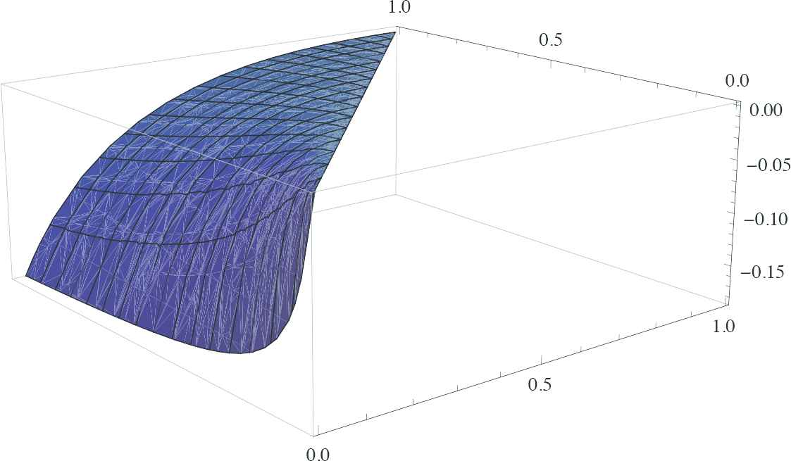
Let us consider a parallel system of n components with lifetime Yi,i=1,2,…,n. Assume that Yi's are independent and identically distributed with a common pdf g(x)=1 and cdf G(x)=x, where 0<x<1. Then X=max{Y1,Y2,…,Yn} be the system lifetime. The cdf of X is F(x)=[G(x)]n=xn,x∈(0,1). Clearly, X≥lrYi,i=1,2,…,n. Further SYi(t1,t2)=ln(t2−t1) and

SX(t1,t2)=n−1n−lnnt2n−t1n−n−1t2n−t1nt2nlnt2−t1nlnt1.

Since analytically it is hard to compare SX(t1,t2) with SYi(t1,t2), therefore we plot the difference SX(t1,t2)−SYi(t1,t2) in Mathematica software (see Figure 3) and notice that this difference is always take negative values in its domain. Hence we conclude that X≤DTEYi. This facts ensure us that a parallel system described above is mostly acceptable than a single component system in DTE-lr order.

The following theorem shows that the orders defined in Definition 6.1 are closed under affine transformations of the form ϕ(t)=at+b, where a>0 and b≥0.

Theorem 6.1

Consider Z1=aX+b and Z2=aY+b, a>0 and b≥0, where X and Y are absolutely continuous random lifetimes of two components. Assume t1>b. If X is mostly acceptable than Y in DTE-lr (DTE-st) order, then Z1 is mostly acceptable in Z2 in DTE-lr (DTE-st) order.

Proof.

Proof follows from Theorem 2.2 and the properties of the orderings given by Definition 1.1. Thus, it is omitted.

7. CONCLUSION

In this paper, we consider Shannon entropy of a doubly truncated random variable and study its properties. We introduce a new order based on doubly truncated entropy and study its connection with other stochastic order. A new class of lifetime distributions based on the doubly truncated entropy is proposed. Characterizations of some life distributions are obtained. Some results on discrete distributions are also addressed here. Finally, based on doubly truncated entropy, how to choose the better system is discussed.

ACKNOWLEDGMENTS

The authors would like to thank the Editor, Associate Editor and the anonymous referees for their careful reading and comments which have improved the presentation of this paper.

REFERENCES

1.B. Efron and V. Petrosian, J. Am. Stat. Assoc., Vol. 94, 1999, pp. 824-834.

2.W.B. Bilker and M.C. Wang, Biometrics, Vol. 52, 1996, pp. 10-20.

3.H. Stovring and M.C. Wang, BMC Med. Res. Methodol., Vol. 7, 2007, pp. 53.

4.H. Zhu and M.C. Wang, Biometrika, Vol. 99, 2012, pp. 345-361.

5.C. Moreira, J. de Una-Alvarez, and I. Van Keilegom, Comput. Stat., Vol. 29, 2014, pp. 1365-1379.

6.C. Shannon, Bell Syst. Tech. J., Vol. 27, 1948, pp. 379-423.

7.S.M. Sunoj, P.G. Sankaran, and S.S. Maya, Commun. Stat. Theory Methods, Vol. 38, 2009, pp. 1441-1452.

8.F. Misagh and G. Yari, Entropy, Vol. 14, 2012, pp. 480-490.

9.C. Kundu, Commun. Stat. Theory Methods, Vol. 46, 2017, pp. 3135-3147.

10.C. Kundu, Commun. Stat. Theory Methods, Vol. 46, 2017, pp. 10594-10606.

11.J. Navarro and J.M. Ruiz, IEEE Trans. Reliab., Vol. 45, 1996, pp. 685-690.

12.M. Shaked and J.G. Shanthikumar, Stochastic Orders, Springer Verlag, New York, NY, USA, 2007.

13.N. Ebrahimi and F. Pellerey, J. Appl. Probab., Vol. 32, 1995, pp. 202-211.

14.A.K. Nanda and P. Paul, Metrika, Vol. 64, 2006, pp. 47-61.

15.R.E. Barlow and F. Proschan, Statistical Theory of Reliability and Life Testing, Holt, Rinehart and Winston, New York, NY, USA, 1975.

16.S. Zacks, Introduction to Reliability Analysis Probability Models and Methods, Springer-Verlag, New York, NY, USA, 1992.

17.C.D. Lai and M. Xie, Stochastic Ageing and Dependence for Reliability, Springer, New York, NY, USA, 2006.

18.N. Ebrahimi, Sankhya, Vol. 58, 1996, pp. 48-57.

19.N. Ebrahimi and S.N.U.A. Kirmani, Stat. Probab. Lett., Vol. 29, 1996, pp. 167-176.

20.M. Nourbakhsh and G. Yari, in Proceedings of the 1st International Electronic Conference Conference on Entropy and its Applications, 2014.

21.M. Khorashadizadeh, A.H. Rezaei Roknabadi, and G.R. Mohtashami Borzadaran, Stat. Probab. Lett., Vol. 83, 2013, pp. 1464-1471.

22.F. Belzunce, J. Navarro, J.M. Ruiz, and Y. Aguila, Metrika, Vol. 59, 2004, pp. 147-161.

23.M. Khorashadizadeh, A.H. Rezaei Roknabadi, and G. R, Commun. Stat. Theory Methods, Vol. 41, 2012, pp. 1105-1115.

24.V. Kumar, R. Thapliyal, and H.C. Taneja, J. Stat. Theory Appl., Vol. 12, 2013, pp. 120-128.

25.G. Asha, I. Elbatal, and C.J. Rejeesh, Commun. Stat. Theory Methods, Vol. 45, 2016, pp. 1081-1098.

<Previous Article In Issue

Download article (PDF)

Next Article In Issue>

Journal: Journal of Statistical Theory and Applications
Volume-Issue: 19 - 2
Pages: 261 - 273
Publication Date: 2020/06/08
ISSN (Online): 2214-1766
ISSN (Print): 1538-7887
DOI: 10.2991/jsta.d.200512.003 How to use a DOI?
Open Access: This is an open access article distributed under the CC BY-NC 4.0 license (http://creativecommons.org/licenses/by-nc/4.0/).

Cite this article

ris enw bib

TY  - JOUR
AU  - Rajesh Moharana
AU  - Suchandan Kayal
PY  - 2020
DA  - 2020/06/08
TI  - Properties of Shannon Entropy for Double Truncated Random Variables and its Applications
JO  - Journal of Statistical Theory and Applications
SP  - 261
EP  - 273
VL  - 19
IS  - 2
SN  - 2214-1766
UR  - https://doi.org/10.2991/jsta.d.200512.003
DO  - 10.2991/jsta.d.200512.003
ID  - Moharana2020
ER  -

download .riscopy to clipboard