
On the Probabilistic Latent Semantic Analysis Generalization as the Singular Value Decomposition Probabilistic Image
- DOI
- 10.2991/jsta.d.200605.001How to use a DOI?
- Keywords
- Singular value decomposition; Probabilistic latent semantic analysis; Nonnegative matrix factorization; Kullback–Leibler divergence
- Abstract
The Probabilistic Latent Semantic Analysis has been related with the Singular Value Decomposition. Several problems occur when this comparative is done. Data class restrictions and the existence of several local optima mask the relation, being a formal analogy without any real significance. Moreover, the computational difficulty in terms of time and memory limits the technique applicability. In this work, we use the Nonnegative Matrix Factorization with the Kullback–Leibler divergence to prove, when the number of model components is enough and a limit condition is reached, that the Singular Value Decomposition and the Probabilistic Latent Semantic Analysis empirical distributions are arbitrary close. Under such conditions, the Nonnegative Matrix Factorization and the Probabilistic Latent Semantic Analysis equality is obtained. With this result, the Singular Value Decomposition of every nonnegative entries matrix converges to the general case Probabilistic Latent Semantic Analysis results and constitutes the unique probabilistic image. Moreover, a faster algorithm for the Probabilistic Latent Semantic Analysis is provided.
- Copyright
- © 2020 The Authors. Published by Atlantis Press SARL.
- Open Access
- This is an open access article distributed under the CC BY-NC 4.0 license (http://creativecommons.org/licenses/by-nc/4.0/).
1. INTRODUCTION
The Probabilistic Latent Semantic Analysis (PLSA) have formal similarities with the Singular Values Decomposition (SVD). The obtained probabilistic factorization admits a matrix representation which can be assimilated to the SVD one. In fact, the original formulation of Hofmann [1] is a probabilistic remake of Latent Semantic Analysis (LSA), which is a direct SVD application introduced by Deerwester et al. [2]. Despite similarities, fundamental differences exist, since every real entries matrix admits the SVD decomposition, but only count data structures (and consequently contingency tables) PLSA decomposes. In fact, the PLSA has been derived from the probability theory, with hard restrictions. The idea of the PLSA is to factorize the co-occurrence table
The work of Hofmann received strong criticism after publishing the main ideas on [1]. One of the most important one is the paper of Blei et al. [3], who pointed out several objections. The most important for the purposes of this manuscript is about the number of parameters of the PLSA model, which grows linearly when new data are added (documents), and the EM algorithm heritage, which has serious computational problems in terms of memory and execution time. Despite the problems, the PLSA is a very effective tool for information retrieval, text and image classification, bioinformatics, unsupervised machine learning, and constitutes a start point of some ideas as the probabilistic clustering. Despite the problems, the number of works using this technique has grown while the computing power increases.
A closely related technique to the PLSA is the Nonnegative Matrix Factorization (NMF). The NMF historically attributed to Chen [4] and extended by Paatero and Taper [5], can be used to solve similar problems to the PLSA in a less restrictive framework. The equivalence among the NMF and the PLSA has been discussed by Gaussier and Goutte [6] and Ding et al. [7], since every nonnegative entries matrix has a probabilistic interpretation under suitable normalization conditions, as is shown in [7], between many others. And advantage of the NMF is the ability to handle more general data structures than the discrete ones, referred by the PLSA. However, the PLSA solves the problem of maximizing the log-likelihood, while the NMF try to find two matrices
While the PLSA practitioners are going on an algorithms competition to achieve good and reasonable fast results, not many theoretical works has been published. Some exceptions are the contributions of Brants [8] who uses the model for inferential purposes. Chaudhuri (2012) relates the diagonal matrix with the Mahalanobis distance [9], and Devarajan et al. [10] discuses several divergences, relating them with probability distributions.
The NMF create a scenario on which it is possible to derive similar equations to the obtained by Hofmann, for a wider data class, into a less restrictive framework. Deriving equations from the NMF with Kullback–Leibler (KL) divergence, ensuring the minimal number of components which guarantees monotonicity as is shown by Latecki et al. [11], and extracting the diagonal matrix as the inertia vector values, we call the formulas obtained in this way general case PLSA equations.
To avoid a bad definite problem or the undesirable effect of local maximums, the iterative procedure in the generalized PLSA factorization is done until the empirical distribution of the obtained product matrices is the same as the original data matrix, both with suitable normalization conditions. Under those assumption is easy to prove that for any nonnegative entries matrix, the singular value decomposition of the Gram–Schmidt orthonormalization (referred to it in the form given in [12, p. 24]) is the same as the generalized PLSA obtained matrices product Gram–Schmidt orthonormalization. At this point is possible to establish the conditions which provides equal results, under the condition of the empirical distributions are reached. Then, the generalized PLSA formulas solves the PLSA (also, classical PLSA) problem too.
The next section is an overview of the main ideas, like the SVD theorem and the LSA, which constitutes the basis to introduce the PLSA as a probabilistic remake. The most fundamental ideas of the NMF and the PLSA formulas are introduced in section 2 and Section 3 is devoted to derive the general case PLSA equations. Other section is devoted to the PLSA and SVD relation in the simplest way we can. Section 5 offers an example of the properties, with a reduced data set. Despite the example is driven with a small dimensions matrix, up to
2. BACKGROUND
2.1. The Singular Value Decomposition
The well-known SVD is a generalization of the elementary lineal algebra Spectral Decomposition Theorem. The SVD states that every matrix
If the rank of
The theoretical and practical consequences of the SVD are vaste. It is the main idea of many of the Multivariate Methods, and provides a geometrical interpretative basis for them. Moreover, the SVD does not involve many calculations and it is implemented in several of the existing programming languages [13, p. 309]. The flexibility and aptitude of the SVD for data analysis highlights the LSA, which can be considered a special interpretation case of the SVD.
On the LSA problem, the matrix
2.2. The PLSA Model
The PLSA model is a probabilistic remake of the LSA, obtained from the frequencies table
The expression Eq. (2) can be written as
The PLSA estimates the probabilities of Eq. (3) maximizing the log-likelihood by using the EM algorithm. For the symmetric formulation is
Hofmann maximizes the expression Eq. (4) by computing the expectation, which is the posterior (E-step)
By switching between Eq. (5) and the group of Eqs. (6–8), until certain condition is achieved, the model is adjusted.
The analogy between Eqs. (6–8) and the given by Eq. (1) is put in the scene when is written [1]
2.3. The NMF Point of View
A closely related PLSA problem is the MFN. It is usually stated as the decomposition of the nonnegative matrix
The problem of the NMF for a matrix
The equivalence between the PLSA and NMF problems needs a diagonal matrix. Gaussier and Goutte [6] shows that introducing diagonal matrices
3. GENERAL CASE EQUATIONS
Equivalent formulas to Eqs. (14) and (15) can be derived from the KL divergence. For
Switching between Eqs. (18) and (19) after initializing, until certain condition is achieved, and assuming convergence in the iterative process, the obtained matrices product of
The pairs of Eqs. (18, 19), and (14, 15) are similar, but not equivalent since the derivation context is different [16, Chap. 3]. In the other hand, the classical KL divergence definition evidences the log-likelihood similitude with the second term of Eq. (17), while the first is a constant. This shows the equivalence between the KL divergence minimization and the EM algorithm. Moreover, the use of the KL divergence has good theoretical properties in a simple framework.
Formal similitude between the Eqs. (18) and (19) and the classical PLSA given by the formulas Eqs. (6–8), requires a diagonal matrix, which plays the role of Eq. (7).
Since the centered matrix of
Simple algebra manipulations
While the SVD dimension reduction problem is bounded by the nonzero eigenvalues, the number of model components is a controversial point within the PLSA, which inherits the EM algorithm problems. There are no restrictions on the number of latent variables (number of nonzero entries in
Each one of the
Only the largest values of
Taking into account that the empirical density of
Proposition 3.1.
The number of model components which ensures that the empirical distribution of
Introducing as a definition to refer the obtained formulas in a more concise way
Definition 3.1
For
4. PROPERTIES
The general case PLSA equations are a merely similitude reformulation of the Eqs. (21–23) with the SVD, if the connection between them is not established. The underlying relation can be seen by taking into account the convergence of the iterative process. Then, if
Proposition 4.1.
The SVD of the orthonormalization (ortogonalization and column normalization) Gram–Schmidt of
Proof.
After orthogonalize and normalize
A direct consequence is, despite the data are rarely orthogonal
Proposition 4.2.
If the columns of
A practical way to ensure the empirical distribution equality
Definition 4.1
The
The degree of adjustment between the characters matrices can be measured with the
Proposition 4.3.
The condition
In practical conditions the zero bound is difficult to achieve, since the matrix
Proposition 4.4.
The matrix
Proof.
If
In this case the maximum is achieved, since from a numerical point of view, when the condition
A similar construction to the given by propositions 4.1–4.4 can be build up for the classical PLSA Eqs. (6–8), when they are written in matrix form, reaching also the maximum. In this case the relation between the classical PLSA model and the general case PLSA equations relies on the significance of the diagonal matrix given by Eqs. (6) and (21), respectively. In this case the relation between
Proposition 4.5.
The expectation of
Proof.
Since
Introducing as a definition the steps to ensure the equality between decompositions
Definition 4.2
The probabilistic SVD image is obtained when the general case PLSA equations reach the limit on which the empirical distributions are the same, except for
And recompiling the previous properties as a compact result, it can be stated
Theorem 4.1.
The probabilistic SVD image, the classical and general case PLSA matrix factorization are equal when
If statistical inference will be done is unique necessary to normalize suitable columns or rows. In this work we go no far on this point.
5. EXAMPLE
This section offers a very simple example. It analyzes the effect of the number of components in the general case PLSA equations on the reached convergence limit, and compares it with the classical PLSA. For this purpose the
Since the number of iterations which are necessary to reach the maximum grows linearly with the data matrix dimension and the number of components, the small data set decathlon is used to drive the example. Included in several R packages, with some differences among them, the selected one is the included in the FactoMineR one [17]. The data are the ranks of elite athletes participants in the Athenas 2012 Olimpic Games men's decathlon competition. Additional reductions are done in the data by selecting
The data can be written as a nonnegative real valued
One must be careful at the moment to ordering the results, if significance will be provided. There are two categories: more is better, which corresponds to the distance achieved for events like jumping or shots, and less is better, which is the case of the time to cover a distance by running. Not always this correspondence occurs, and it should be done in a cautious way in all the cases if significance will be provided, but it is not important for computation purposes. The qualitative matrix
To see how the
| 100 | Long | … | 1500 | |
|---|---|---|---|---|
| LB | MB | … | LB | |
| Karpov | Clay | … | Lorenzo | |
| Averyanov | Sebrle | … | Smirnov | |
| Warners | Karpov | … | Hernu | |
| ⋮ | ⋮ | ⋮ | ⋮ | |
| Schoenbeck | Parkhomenko | … | Korkizoglou | |
| Karpov | Clay | … | Lorenzo | |
| Clay | Sebrle | … | Gomez | |
| Averyanov | Karpov | … | Smirnov | |
| ⋮ | ⋮ | ⋮ | ⋮ | |
| Casarsa | Casarsa | … | Korkizoglou |
Note: Characters matrix
Obtained qualitative matrices of characters.
The comparation between
The objective is to adjust the
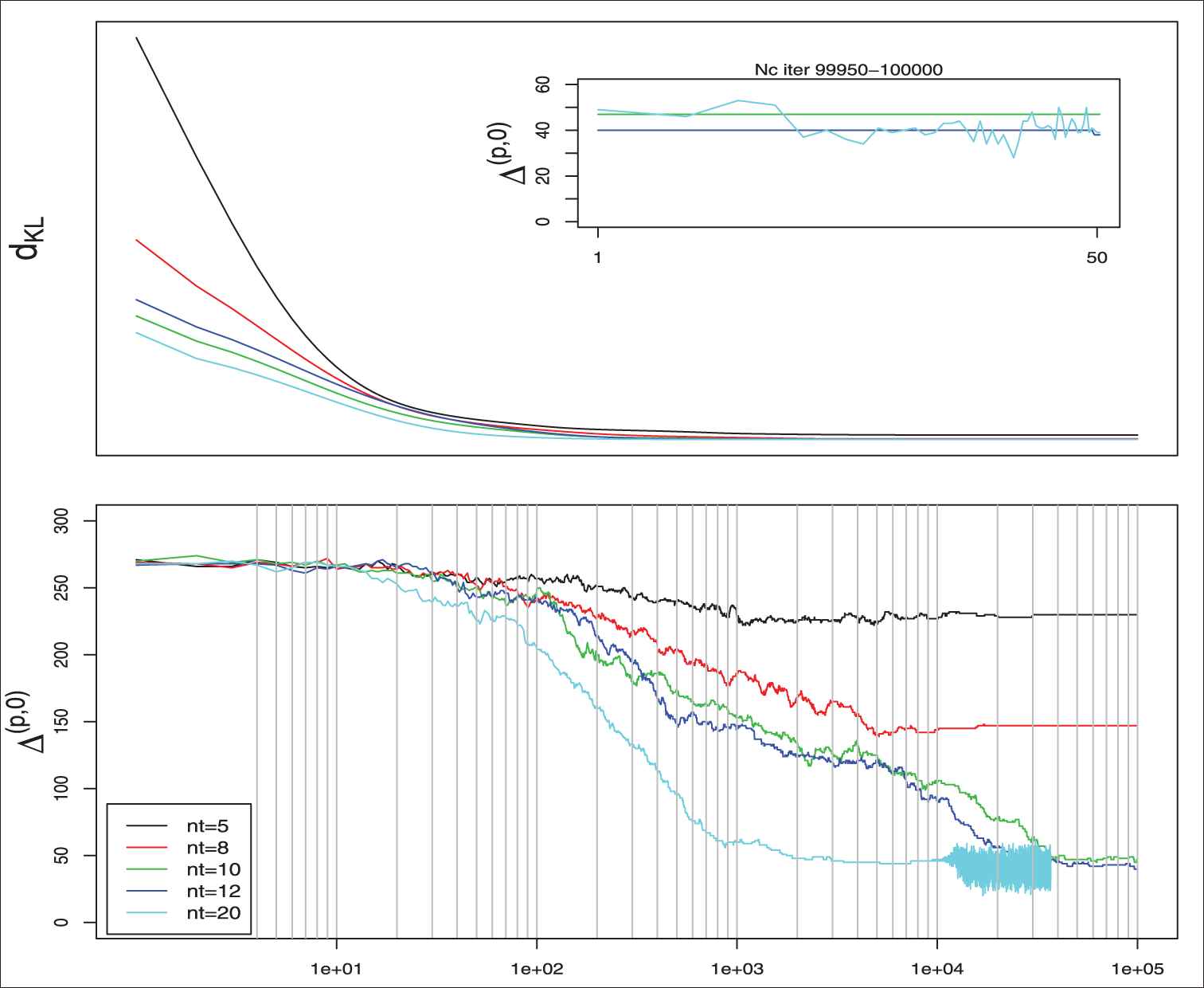
The two figures share the same abscissa axis. The top graphics shows the how decreases the KL divergence as the iterations increases for different number of model components. Initial values are randomized. The bottom figure shows the number of mismatches. When
From a purely computational point of view, the obtained results are compared with the classical PLSA, which offers similar results as those shown in the Figure 1. In this case the PLSA is improperly run, since the data are not multinomial distributed, but the purpose is purely computational. The results are the same, and differences are debt to random initialization conditions. In the Figure 1 it can be seen too how oscillates close to the maximum, and a little more of iterations stabilizes the result. At this point the numerical approximation error is small and lets to reconstruct the original empirical distribution, and if the sums are saved, the original data matrix can be reconstructed (except for the repeated values and labels of the data matrix).
For a enough large number of iterations, it can be seen how the diagonal matrix obtained by the formula (21), which is the estimation of
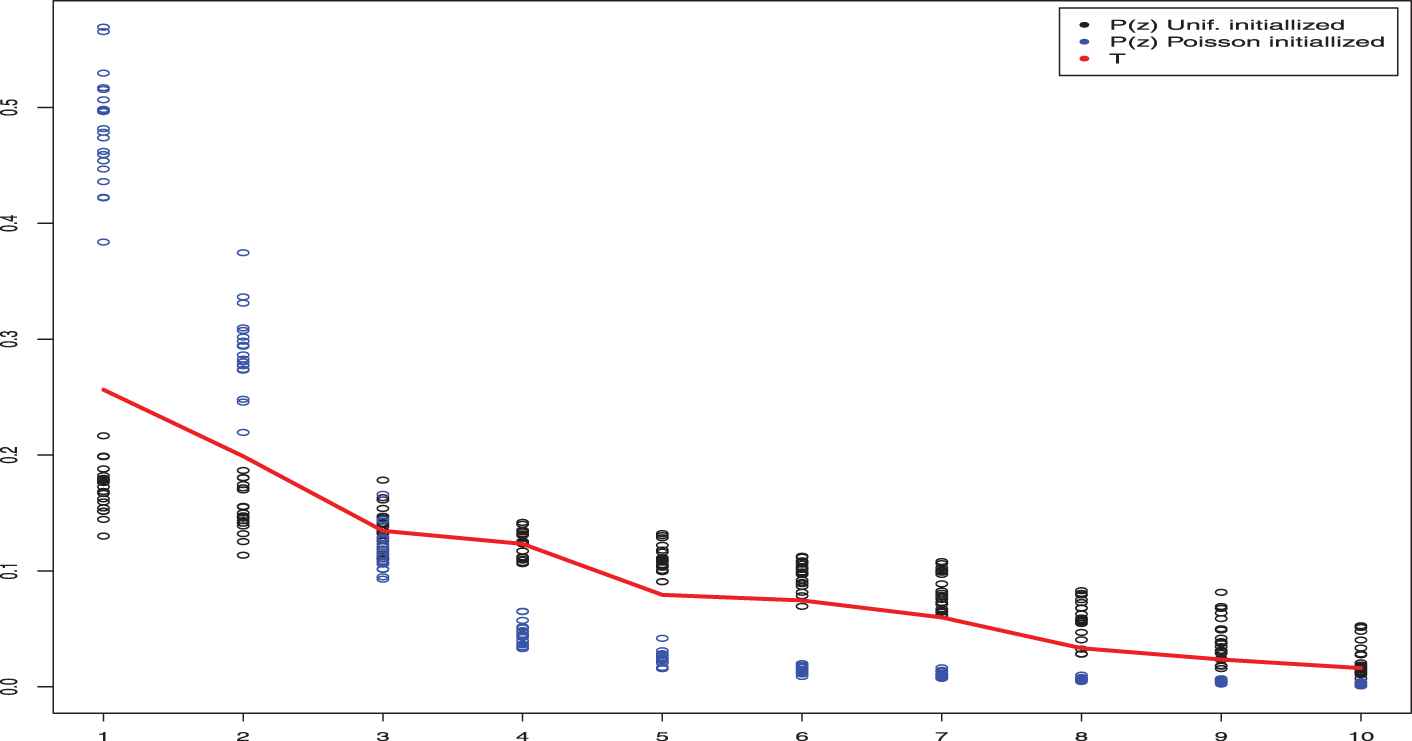
Expected value for P(z) when the classical PLSA algorithm has been initialized under different conditions. The uniform initialized P(z) values has the limit exponential distribution [18, p.157] and the Poisson, under certain conditions is a exponential too [18, p.158]. Both cases are a special selection parameters of a
A not minor consequence of the general case PLSA formulas is the increasing computational speed, as can be seen in table 2. A well-known problem of the PLSA practitioners is the complexity in terms of time and memory. The general case PLSA equations reduces this drawback to a NMF difficulty one. Since the EM algorithm convergence is slow, the KL based too, and it is a consequence of their intimately connection, but the fact to avoid the estimation of the object of Eq. (5), simplifies the operations. It has important consequences, since the final results requires less time. When only in PLSA practical results interest is, a trick is to run Eqs. (18) and (19) with a large number of model components, since the interest relies only in matrices
| Time Cicle (ms) | Total Memory (MB) | |
|---|---|---|
| Classical PLSA | 14,379 | 132.0 |
| Generalized PLSA | 1,350 | 106.6 |
Note: Computations done with a Intel 8.00 GB RAM 2.30 GHz processor.
Speed comparison between classical and generalized Probabilistic Latent Semantic Analysis (PLSA) equations algorithm performance (time for
6. DISCUSSION
The iterative process to obtain the generalized PLSA matrices, minimizes the KL divergence between the object and image matrix. The entries of
Another point to study in more depth are the local basis rotations from a statistical point of view, to ensure the results interchangeability between both points of view. In the euclidean space case, this fact is depth studied, and the consequences are irrelevant, but it is not so clear when talking about probability distributions.
The general case PLSA and the SVD relation has been established for the full rank case. The low rank is used in connection with the problem of dimension reduction. These concepts should be also related for the general case PLSA, to establish the limits and advantages of this similarity, and reveal in a more clear way the achieved convergence limit.
From a purely practical point of view, it is necessary to increase the computational and convergence speeds of the algorithm. The faster iterative procedure with the I-divergence is the basis of many of the current algorithms, but cannot be put in relation with the KL divergence. Necessarily, this leads to establishing the relationship between the KL divergence (or the EM algorithm) with other types of divergences. Therefore, is necessary a broader conceptual base on this field.
7. CONCLUSIONS
From the obtained results, three conclusions can be established. First, the probabilistic SVD image is asymptotically unique and allows to provide inferential sense to descriptive statistical techniques based on the SVD. Second, an algebraic consequence is the total equivalence between the classical PLSA and the general PLSA model (when certain conditions are satisfied). This shows that statistical problems, under suitable conditions, is an algebraic one, under a reliable conceptual basis. Finally, the general case PLSA equations has no distributional hypothesis, and solely restricted to real-valued entries. This leads to estimate under a quantitative basis the optimal number of model components and its significance.
CONFLICT OF INTEREST
No conflict of interest declaration for manuscript title.
AUTHORS' CONTRIBUTIONS
Figuera Pau: Conceptual development and main work. García Bringas Pablo: Professor Garcia Bringas is my Thesis Director, and his inestimable asportation is on fundamental questions and objections, with infinitely patience, to make clear the main ideas.
ACKNOWLEDGMENTS
We would like to show our gratitude to the editor-in-chief Prof. M. Ahsanullah and the unknown referees, for the patience to accept relevant changes once the manuscript was submitted. Without this collaboration, this manuscript would have been impossible to be published.
Footnotes
Also, it can be decomposed as
REFERENCES
Cite this article
TY  - JOUR
AU  - Pau Figuera Vinué
AU  - Pablo García Bringas
PY  - 2020
DA  - 2020/06/19
TI  - On the Probabilistic Latent Semantic Analysis Generalization as the Singular Value Decomposition Probabilistic Image
JO  - Journal of Statistical Theory and Applications
SP  - 286
EP  - 296
VL  - 19
IS  - 2
SN  - 2214-1766
UR  - https://doi.org/10.2991/jsta.d.200605.001
DO  - 10.2991/jsta.d.200605.001
ID  - Vinué2020
ER  -