
The Odd Log-Logistic Geometric Family with Applications in Regression Models with Varying Dispersion
- DOI
- 10.2991/jsta.d.190818.003How to use a DOI?
- Keywords
- Geometric family; Censored data; Maximum likelihood estimation; Odd log-logistic family; Regression model; Varying dispersion
- Abstract
We obtain some mathematical properties of a new generator of continuous distributions with two additional shape parameters called the odd log-logistic geometric family. We present some special models and investigate the asymptotes and shapes. The family density function can be expressed as a linear combination of exponentiated densities based on the same baseline distribution. We derive a power series for its quantile function. We provide explicit expressions for the ordinary and incomplete moments and generating function. We estimate the model parameters by maximum likelihood. We propose a useful regression model by varying the dispersion parameter to fit real data. We illustrate the potentiality of the proposed models by means of three real data sets.
- Copyright
- © 2019 The Authors. Published by Atlantis Press SARL.
- Open Access
- This is an open access article distributed under the CC BY-NC 4.0 license (http://creativecommons.org/licenses/by-nc/4.0/).
1. INTRODUCTION
Recent developments on univariate continuous distributions have been focused to define new families by adding shape parameters to control skewness, kurtosis and tail weights, providing great flexibility in modeling skewed data in practice, including the two-piece approach introduced by Hansen [1] and the generators pioneered by Eugene et al. [2], Cordeiro and de Castro [3], Alexander et al. [4] and Cordeiro et al. [5]. Many subsequent articles apply these techniques to induce skewness into well-known symmetric distributions such as the symmetric Student t. For a review, see Aas and Haff [6].
In the last few years, new classes of distributions were proposed, for example, the generalized Weibull family by Cordeiro et al. [7], the exponentiated G Poisson model (Gomes et al., [8]), the Poisson-X family presented by Tahir et al. [9], the extended-G geometric family by Cordeiro et al. [10], the generalized odd half-Cauchy class by Cordeiro et al. [11] and the generalized odd log-logistic (LL) family studied by Cordeiro et al. [12].
In this work, we introduce a new class of distributions called the odd log-logistic geometric-G (“OLLG-G” for short) family with two additional shape parameters in order to attract wider applications in reliability, biology and other research areas, and study some of its mathematical properties. The new family can extend several common models such as the normal and Weibull distributions by adding two extra parameters to a parent G. The proposed family is an extension of that one introduced recently by Gleaton and Lynch [13].
One way to study the effects of the explanatory variables on the lifetime or survival time is through a regression location-scale model, also known as the accelerated lifetime model. Regression models can be proposed in different forms in survival analysis, for example, Hashimoto et al. [14] defined the long-term survival model with interval-censored data. Ortega et al. [15] defined a power series beta Weibull regression model for predicting breast carcinoma, Lanjoni et al. [16] proposed the extended Burr XII regression model, Ortega et al. [17] introduced the odd Birnbaum-Saunders regression model and, more recently, Ramires et al. [18] predicted the cure rate of breast cancer using a regression model with four regression structures. In this paper, we develop a log-linear model using a new distribution called the log-odd log-logistic geometric Weibull (“LOLLG-W” for short). The new regression model by varying the dispersion parameter can be applied to censored data since it represents a parametric family of models that includes as sub-models several widely-known regression models and therefore can be used more effectively in the analysis of survival data.
This paper is organized as follows: In Section 2, we define the OLLG-G family and propose some new distributions. In Section 3, we derive useful expansions for the new family. In Section 4, we present moments and quantile and generating functions. Maximum likelihood estimation of the model parameters and various simulations for different parameter settings and sample sizes are performed in Section 5. In Section 6, we define a regression model of location-scale form with varying dispersion. In Section 7, we provide some applications. Section 8 offers some concluding remarks.
2. MODEL DEFINITION
Gleaton and Lynch [13], da Cruz et al. [19], Braga et al. [20] and Cordeiro et al. [12] studied a class of distributions called the odd log-logistic (“OLLG-G”) family with applications in different areas. Given a continuous baseline cumulative distribution function (cdf)
Thus, the parameter
Suppose that
Then, the probability density function (pdf) of the
The cdf corresponding to (3) is given by
Henceforth, a random variable
2.1. Special Models
We present two special cases of the new family: the OLLG-Weibull (OLLG-W) and OLLG-normal (OLLG-N) distributions. First, the OLLG-W distribution is defined from (3) by taking
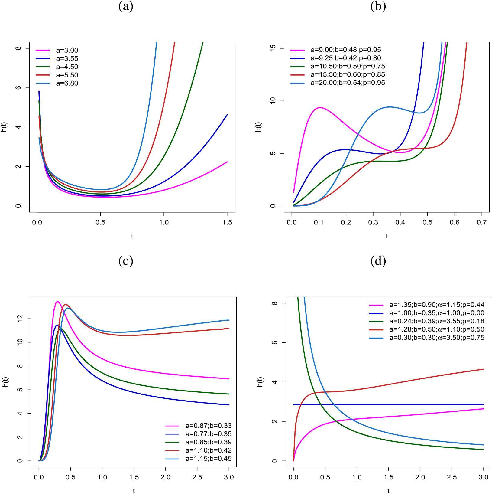
For Plots of the odd log-logistic geometric (OLLG)-Weibull density function for some parameter values. (a) Fixed. Plots of the odd log-logistic geometric (OLLG)-Weibull hazard function for some parameter values. (a) Fixed.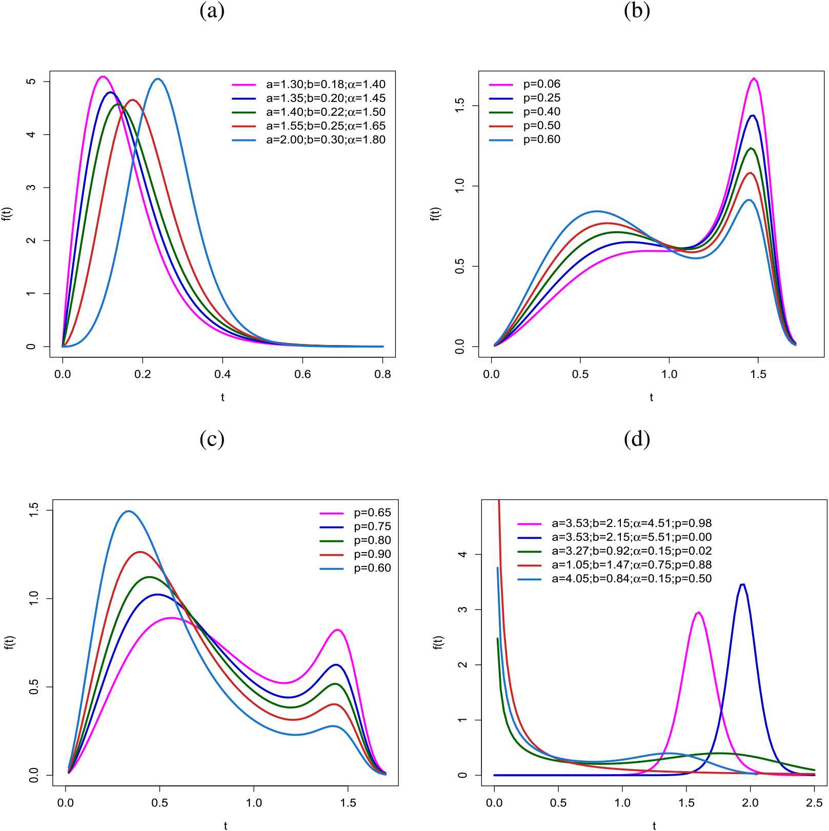
Second, the OLLG-N distribution is defined from (3) by taking
Its density function is given by
For
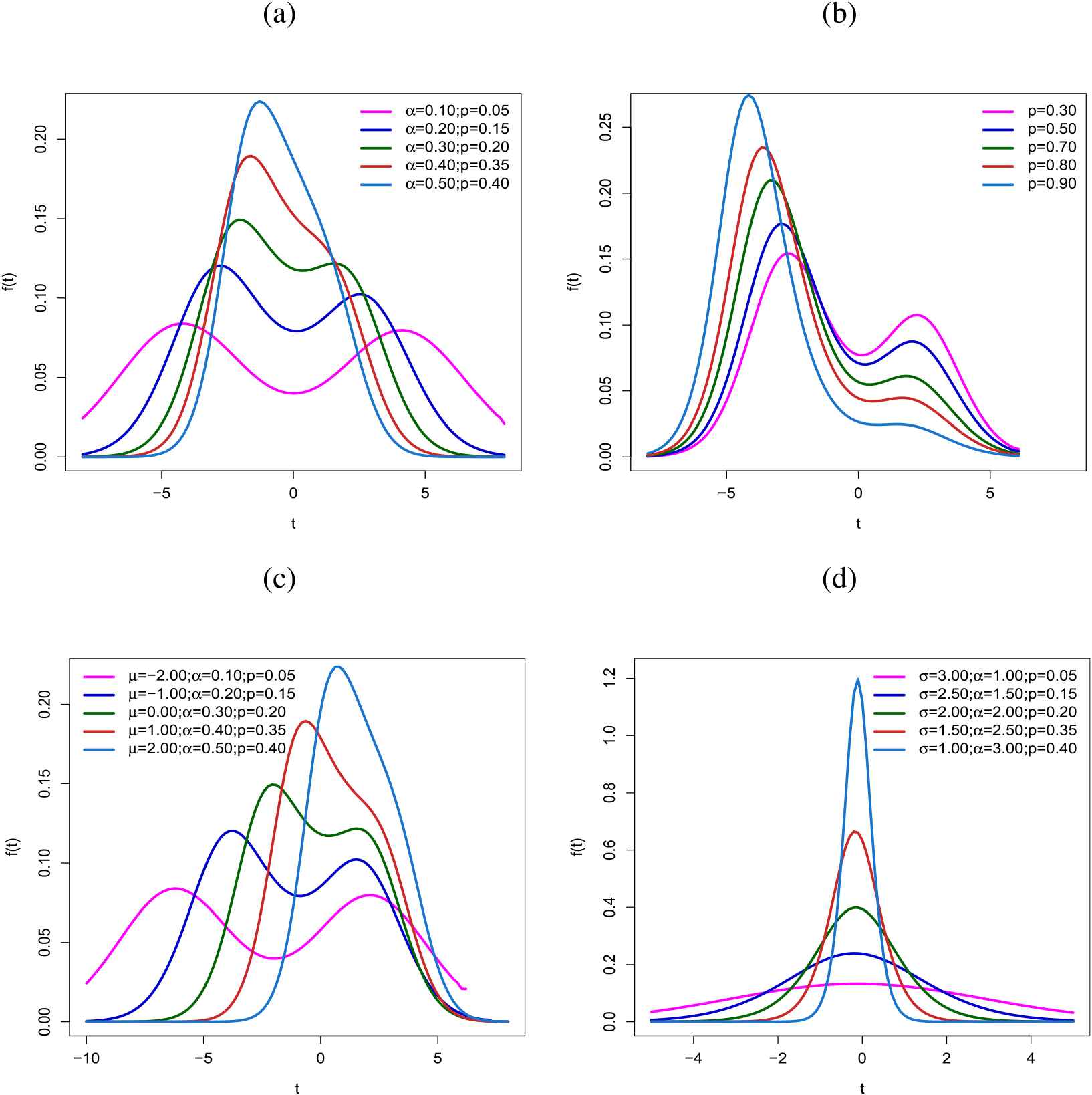
Plots of the odd log-logistic geometric (OLLG)-normal density function for some parameter values. (a) Fixed.
3. USEFUL EXPANSION
Theorem 3.1.
Let
Here,
Proof.
We consider the power series
Thus, we can rewrite (4) using (8) as
Further, for
Combining (9) and (10), we obtain
(7) follows from the ratio of two power series in the last equation.
Corollary 3.1.
The pdf of
Theorem 3.1 and Corollary 3.1 are the main results of this section.
4. MATHEMATICAL PROPERTIES
4.1. Quantile Function
(4) has tractable properties especially for simulations, since the quantile function (qf) of
Figures 4(a) and 4(b) display some plots of the OLLG-W kurtosis and skewness for some parameter values, respectively. We have positive kurtosis and positive and negative skewness. These plots reveal the flexibility of the proposed family with respect to the skewness.
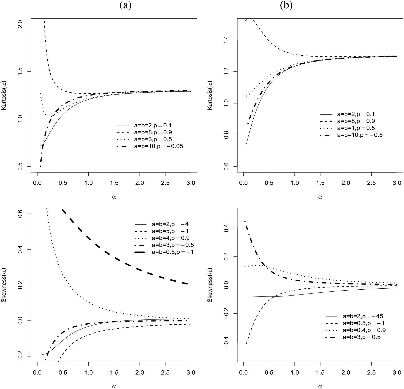
Plots of the kutosis and skewness of the odd log-logistic geometric-Weibull (OLLG-W) and odd log-logistic geometric-normal (OLLG-N) models for some parameter values.
4.2. Moments
In this section, we obtain the ordinary and incomplete moments of
Expressions for moments of several exp-G distributions are given in Nadarajah and Kotz [23].
The
The large number of applications of the ordinary and incomplete moments are well-known in the literature.
4.3. Generating Function
The moment generating function (mgf)
Thus,
5. MAXIMUM LIKELIHOOD ESTIMATION
The parameters of the OLLG-G family are estimated by maximum likelihood from complete samples only. Let
Let
The asymptotic distribution of
We can compute the maximum values of the unrestricted and restricted log-likelihoods to obtain likelihood ratio (LR) statistics for testing some sub-models of the OLLG-
So, we can construct LR statistics to check if the fit using the OLLG-G distribution is statistically “superior” to a fit using the OLL-G, and geometric-G family for a given data set. In any case, hypothesis tests of the type
5.1. Simulation Study
In this section, we assess the finite sample performance of the MLEs in the OLLG-W and OLLG-N distributions, respectively, by varying the true parameter and the sample size
First, we consider the OLLG-W model under some parametric variation structure and measure the effects of the MLEs
| AEs |
MSEs |
||||||||
|---|---|---|---|---|---|---|---|---|---|
| (3.53,2.15,0.35,0.25) | 80 | 4.3287 | 2.2555 | 0.3277 | 0.2963 | 4.0096 | 0.1164 | 0.0088 | 0.0538 |
| 150 | 3.8360 | 2.2012 | 0.3421 | 0.2667 | 0.8711 | 0.0542 | 0.0046 | 0.0336 | |
| 300 | 3.6832 | 2.1767 | 0.3464 | 0.2566 | 0.3894 | 0.0320 | 0.0023 | 0.0236 | |
| (11.5,1.25,0.21,0.60) | 80 | 13.5820 | 1.2582 | 0.1993 | 0.5932 | 28.4536 | 0.0049 | 0.0043 | 0.0193 |
| 150 | 12.4670 | 1.2547 | 0.2041 | 0.5964 | 8.8640 | 0.0023 | 0.0018 | 0.0095 | |
| 300 | 11.9975 | 1.2537 | 0.2068 | 0.6020 | 3.4259 | 0.0010 | 0.0009 | 0.0043 | |
| (5.50,1.25,0.21,0.90) | 80 | 9.4602 | 1.2924 | 0.1806 | 0.8895 | 51.0649 | 0.0649 | 0.0183 | 0.0075 |
| 150 | 7.1223 | 1.2703 | 0.2020 | 0.8929 | 13.8234 | 0.0379 | 0.0124 | 0.0025 | |
| 300 | 6.2040 | 1.2623 | 0.2042 | 0.8988 | 4.1319 | 0.0159 | 0.0041 | 0.0007 | |
OLLG-W, odd log-logistic geometric-Weibull; AE, average estimate; MSE, mean square error.
Simulations for the OLLG-W model.
Next, we consider the OLLG-N model to measure both the effects of the MLEs
| AEs |
MSEs |
||||||||
|---|---|---|---|---|---|---|---|---|---|
| (2.00,1.00,0.50,0.40) | 80 | 2.0534 | 1.0035 | 0.5074 | 0.3733 | 0.4381 | 0.2232 | 0.0971 | 0.0577 |
| 150 | 2.0120 | 0.9893 | 0.5022 | 0.3722 | 0.1966 | 0.1627 | 0.0779 | 0.0550 | |
| 300 | 2.0080 | 1.0007 | 0.5026 | 0.3885 | 0.0548 | 0.0391 | 0.0186 | 0.0217 | |
| (0.00,0.75,0.15,0.90) | 80 | −0.0036 | 0.8056 | 0.1945 | 0.8854 | 3.5090 | 0.3043 | 0.0405 | 0.0031 |
| 150 | −0.0357 | 0.7817 | 0.1752 | 0.8938 | 0.2753 | 0.0713 | 0.0137 | 0.0015 | |
| 300 | −0.0064 | 0.7602 | 0.1606 | 0.8962 | 0.0953 | 0.0309 | 0.0055 | 0.0012 | |
| (−1.00,1.00,0.20,0.15) | 80 | −0.9114 | 1.0140 | 0.2142 | 0.2139 | 0.1436 | 0.0944 | 0.0119 | 0.0304 |
| 150 | −0.9345 | 1.0180 | 0.2105 | 0.1840 | 0.0823 | 0.0475 | 0.0059 | 0.0200 | |
| 300 | −0.9462 | 1.0097 | 0.2057 | 0.1853 | 0.0405 | 0.0199 | 0.0023 | 0.0136 | |
OLLG-N, odd log-logistic geometric-normal; AE, average estimate; MSE, mean square error.
Simulations for the OLLG-N model.
6. THE LOG-OLLG-W REGRESSION MODEL WITH VARYING DISPERSION
In this section, we define a location-scale regression model with varying dispersion based on the OLLG-W distribution called the LOLLG-W regression model with varying dispersion. We consider a classic analysis for this regression model and the inferential part is carried out using the asymptotic distribution of the MLEs.
Henceforth,
The survival function of
The random variable
A parametric model that provides a good fit to lifetime data tends to yield more precise estimates of the quantities of interest. Based on the LOLLG-W density, we propose a linear location-scale regression model with varying dispersion for the response variable
The LOLLG-W regression model with varying dispersion (17) opens new possibilities for fitting many different types of data. The LOLL-W regression model with varying dispersion is a special case when
Consider a sample
The asymptotic distribution of
7. APPLICATIONS
In this section, we provide three applications to real data to prove empirically the flexibility of the OLLG-W and OLLG-N models. The computations are performed using the R software. In the first application, we compare the OLLG-N with geometric normal (Geo-N), OLL-N, Kumaraswamy normal (Kw-N), exponentiated normal (EN), gamma normal (GN) and normal distributions. In the second application, we compare the OLLG-W model with the geometric Weibull (Geo-W), OLL-W, Kumaraswamy Weibull (Kw-W), exponentiated Weibull (EW), gamma Weibull (GW), flexible Weibull (FW) and Weibull models. In the third application, a regression model is investigated considering the OLLG-W distribution.
The FW distribution Bebbington et al. [25], having two parameters
The gamma-
The Kumaraswamy-
The exponentiated-
We report the MLEs (and the corresponding standard errors in parentheses) of the model parameters and the following goodness-of-fit measures: Cramr-von Mises (
7.1. Uncensored Data
First, we consider two uncensored data sets described below.
Guinea pig survival times (E1): The data refer to survival times on days of
Voltage data (E2): The data set was studied by Meeker and Escobar ([27], p. 383), which gives the times of failure and running times for a sample of devices from a field-tracking study of a larger system. At a certain point in time,
To analyze the E1 data, we consider the OLLG-N model and for the E2 data we take the OLLG-W model. Table 3 gives a descriptive summary for these data showing different degrees of skewness and kurtosis. We note that the E1 data have positive asymmetry and kurtosis and that the E2 data have negative values for both.
| Data | Mean | Median | SD | Skewness | Kurtosis | Min. | Max. |
|---|---|---|---|---|---|---|---|
| E1 | 141.8 | 102.5 | 109.2086 | 2.4631 | 6.0742 | 43.0 | 598.0 |
| E2 | 177.0 | 196.5 | 144.9922 | −0.2699 | −1.6416 | 2.0 | 300.0 |
Descriptive statistics for the two data sets.
Tables 4 and 5 list the MLEs and standard errors (in parentheses) of the parameters of the fitted models to both data sets. The values of the statistics are presented in Table 6 to verify the goodness-of-fit of the models under study. The results in this table indicate that the OLLG-N and OLLG-W models have the lowest values of these statistics among all fitted models to both data sets.
| Model | ||||
|---|---|---|---|---|
| OLLG-N | 374.7037 | 30.7166 | 0.1058 | 0.9837 |
| (0.0852) | (0.0859) | (0.0106) | (0.0080) | |
| OLL-N | 125.6653 | 246.6182 | 3.1757 | (0) |
| (9.6367) | (63.4368) | (0.9672) | (−) | |
| Geo-N | 395.4403 | 106.1374 | (1) | 0.9957 |
| (52.3187) | (10.9766) | (−) | (0.0040) | |
| Kw-N | −335.3843 | 132.0140 | 961.8518 | 0.4019 |
| (0.2126) | (0.2141) | (194.1546) | (0.0539) | |
| EN | −500.6958 | 209.3812 | 528.9657 | 1 |
| (0.0002) | (0.0244) | (0.0852) | (−) | |
| Normal | 141.8156 | 108.5312 | 1 | 1 |
| (12.7905) | (9.0547) | (−) | (−) | |
| GN | −99.4173 | 125.2552 | 3.9278 | |
| (48.7530) | (9.6677) | (0.8960) | ||
OLLG-N, odd log-logistic geometric-normal; MLE, maximum likelihood estimate; OLL-N, odd log-logistic normal; Geo-N, geometric normal; Kw-N, Kumaraswamy normal; EN, exponentiated normal; GN, gamma normal; OLLG-W, odd log-logistic geometric-Weibull; OLL-W, odd log-logistic Weibull; Geo-W, geometric Weibull; Kw-W, Kumaraswamy Weibull; EW, exponentiated Weibull, GW, gamma Weibull, FW, flexible Weibull.
MLEs of the model parameters for the E1 data set.
| Model | ||||
|---|---|---|---|---|
| OLLG-W | 18.8383 | 247.9113 | 0.0506 | 0.1864 |
| (0.0008) | (0.0008) | (0.0075) | (0.00024) | |
| OLL-W | 10.5453 | 218.1834 | 0.0772 | (0) |
| (0.0398) | (0.0407) | (0.0115) | (−) | |
| Geo-W | 1.2650 | 188.0544 | (1) | |
| (0.0068) | (0.0246) | (−) | ||
| Kw-W | 71.1698 | 295.9313 | 0.0052 | 0.2713 |
| (22.2411) | (2.8993) | (0.0024) | (0.0755) | |
| EW | 20.2227 | 10228.0700 | 0.0109 | 1 |
| (0.0046) | (109.1352) | (0.0019) | (−) | |
| Weibull | 1.2650 | 188.0544 | 1 | 1 |
| (0.2044) | (28.2172) | (−) | (−) | |
| GW | 7.0283 | 351.5713 | 0.1282 | |
| (0.0025) | (0.0026) | (0.0231) | ||
| FW | 0.0032 | 15.8889 | ||
| (0.0004) | (5.2696) | |||
MLE, maximum likelihood estimate; OLLG-W, odd log-logistic geometric-Weibull; OLL-W, odd log-logistic Weibull; Geo-W, geometric Weibull; Kw-W, Kumaraswamy Weibull; EW, exponentiated Weibull, GW, gamma Weibull, FW, flexible Weibull.
MLEs of the model parameters for the E2 data set.
| E1 Data |
|||||||
|---|---|---|---|---|---|---|---|
| Model | AIC | CAIC | BIC | HQIC | |||
| OLLG-N | 820.3 | 820.9 | 829.4 | 823.9 | 0.3636 | 2.0453 | 0.1119 |
| OLL-N | 865.1 | 865.4 | 871.9 | 867.8 | 0.9985 | 5.7098 | 0.1568 |
| Geo-N | 832.8 | 833.1 | 839.6 | 835.5 | 0.5186 | 3.0225 | 0.1182 |
| Kw-N | 833.8 | 833.4 | 841.9 | 836.4 | 0.5292 | 3.1417 | 0.1914 |
| EN | 843.9 | 844.3 | 850.8 | 846.6 | 0.7104 | 4.1636 | 0.1830 |
| Normal | 883.1 | 883.3 | 887.7 | 884.9 | 1.3648 | 7.5981 | 0.2310 |
| GN | 879.1 | 879.5 | 886.0 | 881.9 | 1.2726 | 7.1386 | 0.2277 |
| E2 Data | |||||||
| Model | AIC | CAIC | BIC | HQIC | |||
| OLLG-W | 331.4 | 333.0 | 337.0 | 333.2 | 0.0808 | 0.7022 | 0.1543 |
| OLL-W | 339.8 | 340.7 | 344.0 | 341.1 | 0.0850 | 0.7955 | 0.1688 |
| Geo-W | 374.6 | 375.5 | 378.8 | 375.9 | 0.3035 | 1.8208 | 0.2192 |
| Kw-W | 331.5 | 333.1 | 337.2 | 333.3 | 0.1129 | 0.9476 | 0.1494 |
| EW | 437.6 | 438.5 | 441.8 | 438.9 | 0.3701 | 2.1273 | 0.5391 |
| Weibull | 372.6 | 373.0 | 375.4 | 373.5 | 10.7180 | 56.4562 | 0.9987 |
| GW | 359.8 | 360.7 | 364.0 | 361.1 | 0.1963 | 1.2839 | 0.2277 |
| FW | 387.6 | 388.0 | 390.4 | 388.5 | 0.3246 | 2.0498 | 0.3942 |
OLLG-N, odd log-logistic geometric-normal; OLL-N, odd log-logistic normal; Geo-N, geometric normal; Kw-N, Kumaraswamy normal; EN, exponentiated normal; GN, gamma normal; OLLG-W, odd log-logistic geometric-Weibull; OLL-W, odd log-logistic Weibull; Geo-W, geometric Weibull; Kw-W, Kumaraswamy Weibull; EW, exponentiated Weibull, GW, gamma Weibull, FW, flexible Weibull.
Goodness-of-fit for the two data sets.
A comparison of the proposed distributions with some of their sub-models using LR statistics is provided in Table 7. The
| E1 Data |
||||
|---|---|---|---|---|
| Models | Hypotheses | Statistic |
||
| OLLG-N vs Normal | 7.0 | 0.0301 | ||
| OLLG-N vs OLL-N | 6.2 | 0.0121 | ||
| OLLG-N vs Geo-N | 4.0 | 0.0455 | ||
| E2 Data | ||||
| OLLG-W vs Weibull | 6.2 | 0.0430 | ||
| OLLG-W vs OLL-W | 3.5 | 0.0604 | ||
| OLLG-W vs Geo-W | 6.1 | 0.0131 | ||
OLLG-N, odd log-logistic geometric-normal; OLL-N, odd log-logistic normal; Geo-N, geometric normal; OLLG-W, odd log-logistic geometric-Weibull; OLL-W, odd log-logistic Weibull; Geo-W, geometric Weibull; LR, likelihood ratio.
LR tests for the two data sets.
In order to assess if the model is appropriate, plots of the fitted OLLG-N, Geo-N, Kw-N and normal density functions are displayed in Figure 5(a) and survival functions and the plots of the empirical distributions are displayed in Figure 5(b). Figure 6(a) provides plots of the fitted density functions of the OLLG-W, OLL-W, Kw-N and Weibull models and Figure 6(b) gives the survival functions and the plots to the empirical distributions. These plots indicate that the OLLG-N and OLLG-W distributions provide better fits to the current data sets.
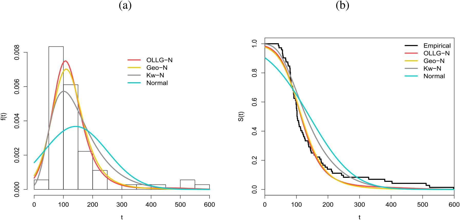
(a) Estimated densities of the odd log-logistic geometric-normal (OLLG-N), geometric normal (Geo-N), Kumaraswamy normal (Kw-N) and Normal models for E1 data. (b) Estimated survival functions of the OLLG-N, Geo-N, Kw-N and Normal models for E1 data.
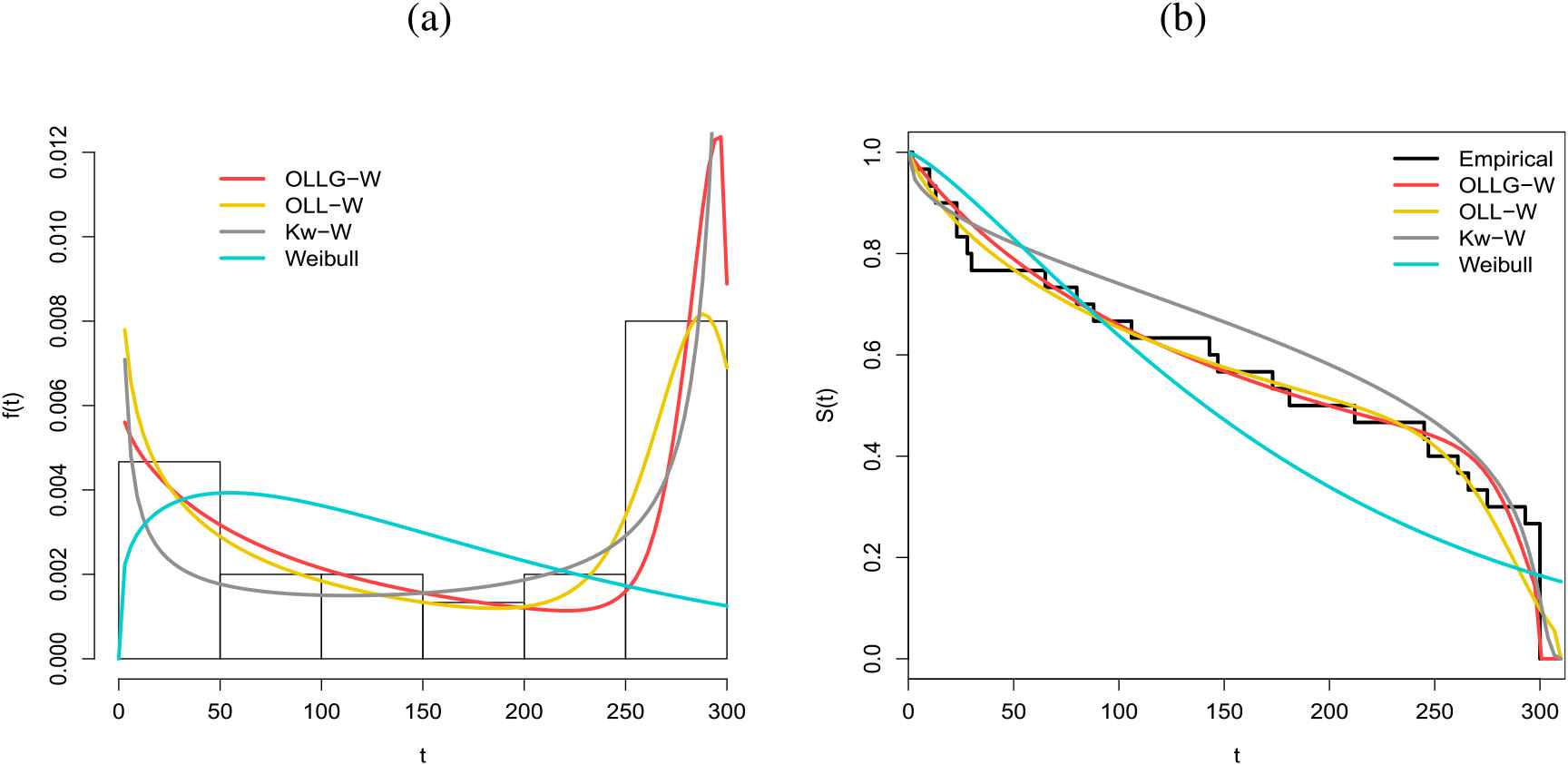
(a) Estimated densities of the odd log-logistic geometric-Weibull (OLLG-W), odd log-logistic Weibull (OLL-W), Kumaraswamy Weibull (Kw-W) and Weibull models for E2 data. (b) Estimated survival functions of the OLLG-W, OLL-W, Kw-W and Weibull models for E2 data.
7.2. Regression Model with Varying Dispersion for Life Expectancy Data
The data were analyzed by Weindruch et al. [28] who compared the life expectancy of field mice under different diets. The authors randomly assigned 244 mice to one of four dietary treatments. The data are available in asbio package of the R software, which contains a data frame with 244 observations on the following two variables:
Exploratory analysis for life expectancy data
Here, we perform an exploratory analysis of these data. Table 8 gives a descriptive summary of the data showing different degrees of skewness and kurtosis. In Figure 7(a) the boxplot of the response variable is shown and in Figure 7(b) the box-plots considering the treatment levels.
Mean Median SD Skewness Kurtosis Min. Max. General 40.88 42.30 8.1321 −0.5547 −0.3514 17.90 54.60 N/N85 32.69 33.10 5.1252 −1.0390 1.0485 17.90 42.30 N/R40 45.12 46.05 6.7034 −1.1755 2.0750 19.60 54.60 N/R50 42.30 43.90 7.7681 −0.9814 0.2534 18.60 51.90 R/R50 40.88 42.30 6.6831 −0.9005 0.1414 24.20 50.70 Table 8Descriptive statistics for the life expectancy data.
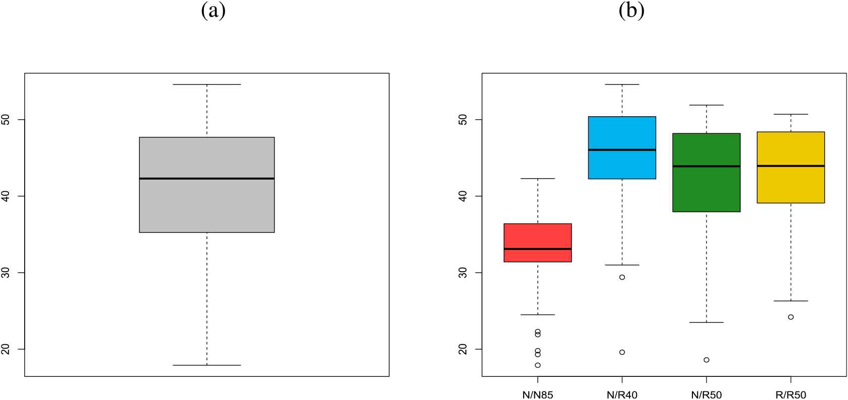 Figure 7
Plots of the response variable. (a) General response variable. (b) Variable response per treatment level.
Table 9 lists the MLEs and standard errors between parentheses of the parameters of the fitted models to the current data. The values of the statistics are given in Table 10 to verify the goodness-of-fit of the fitted models. The results indicate that the OLLG-W model has the lowest values of these statistics among all fitted models to the data.
Model OLLG-W 16.6162 46.1443 0.3669 0.4177 (2.8540) (0.8573) (0.0564) (0.2076) OLL-W 12.1710 44.2047 0.4414 (0) (1.4587) (0.4768) (0.0629) (−) Geo-W 6.1866 44.1086 (1) 0.0002 (0.3245) (0.4805) (−) (0.0091) Kw-W 45.2322 54.1885 0.1038 1.8377 (13.7890) (1.4377) (0.0551) (0.4821) EW 20.1619 50.6639 0.2035 1 (5.5796) (0.8541) (0.0674) (−) Weibull 6.1866 44.1076 1 1 (0.3243) (0.4791) (−) (−) GW 21.8598 51.7215 0.1875 (2.0613) (0.3878) (0.0232) FW 0.0686 132.8122 (0.0034) (7.5067) MLE, maximum likelihood estimate; Kw-N, Kumaraswamy normal; OLLG-W, odd log-logistic geometric-Weibull; OLL-W, odd log-logistic Weibull; Geo-W, geometric Weibull; Kw-W, Kumaraswamy Weibull; EW, exponentiated Weibull, GW, gamma Weibull, FW, flexible Weibull.
Table 9MLEs of the model parameters for the life expectancy data.
Model AIC CAIC BIC HQIC OLLG-W 1676.5 1676.6 1690.5 1682.1 0.0388 0.2610 0.0365 OLL-W 1678.8 1678.8 1689.3 1683.0 0.1152 0.6285 0.0619 Geo-W 1702.1 1702.2 1712.6 1706.3 0.2701 1.7463 0.0894 Kw-W 1683.5 1683.6 1697.5 1689.1 0.1352 0.7567 0.0537 EW 1684.8 1684.9 1695.3 1689.1 0.1949 1.0666 0.0578 Weibull 1700.1 1700.2 1708.1 1702.9 25.4435 125.1121 0.9899 GW 1685.0 1685.1 1695.5 1689.3 0.1996 1.0912 0.0583 FW 1700.6 1700.6 1707.6 1703.4 0.2583 1.7219 0.0910 OLLG-W, odd log-logistic geometric-Weibull; OLL-W, odd log-logistic Weibull; Geo-W, geometric Weibull; Kw-W, Kumaraswamy Weibull; EW, exponentiated Weibull, GW, gamma Weibull, FW, flexible Weibull.
Table 10Goodness-of-fit measures for the life expectancy data.
A comparison of the proposed distributions with some of their sub-models using LR statistics is given in Table 11. The OLL-W model can be considered a more competitive model to the OLLG-W model, because the corresponding
Models Hypotheses Statistic OLLG-W vs Weibull 5.25 0.0720 OLLG-W vs OLL-W 1.60 0.1968 OLLG-W vs Geo-W 5.26 0.0217 OLLG-W, odd log-logistic geometric-Weibull; OLL-W, odd log-logistic Weibull; Geo-W, geometric Weibull.
Table 11LR tests for the life expectancy data.
In order to assess if the model is appropriate, plots of the fitted OLLG-W, OLL-W, Kw-W and Weibull density functions are displayed in Figure 8(a). The estimated survival functions and the plots of the empirical distributions are displayed in Figure 8(b). They indicate that the OLLG-W distribution is gives a good fit to the corresponding data set, thus capturing a slight bimodality with left asymmetry.
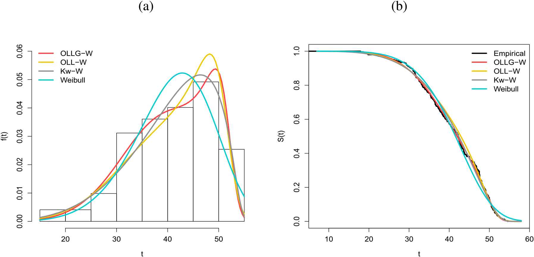 Figure 8
(a) Estimated densities of the odd log-logistic geometric-Weibull (OLLG-W), odd log-logistic Weibull (OLL-W), Kumaraswamy Weibull (Kw-W) and Weibull models for the life expectancy data. (b) Estimated survival functions of the OLLG-W, OLL-W, Kw-W and Weibull models and the empirical cdf for the life expectancy data.
Regression model for life expectancy data
The LOLLG-W regression model for the life expectancy data can be expressed as follows
whereThe MLEs for the LOLLG-W model are presented in Table 12. Thus, when establishing a significance level of 5%, we note that the regression model with varying dispersion capture significant difference between the levels of the diets.
Regression model with constant dispersion Regression model with varying dispersion Parameter Estimate SE Parameter Estimate SE 0.0738 0.0082 − 0.5276 0.0729 − 0.5194 0.0722 − 0.00006 0.0063 − 0.0285 0.0075 − 3.8373 0.0141 3.8337 0.0139 −0.2883 0.0175 −0.2887 0.0181 0.0046 0.0182 0.8006 −0.0183 0.0168 0.2771 −0.0431 0.0237 0.0702 −0.0078 0.0167 0.6408 −2.6363 0.1201 −0.2864 0.1337 0.0331 0.5276 0.1272 0.0197 Table 12MLEs, SEs and
In order to assess if the model is appropriate, the plots comparing the empirical survival function and estimated survival function for the LOLLG-W regression model are displayed in Figures 9(a) and 9(b). These plots indicate that the LOLLG-W regression model with varying dispersion provides a better fit to the data set in Figure 9(b) compared to the homoscedastic regression model Figure in 9(a).
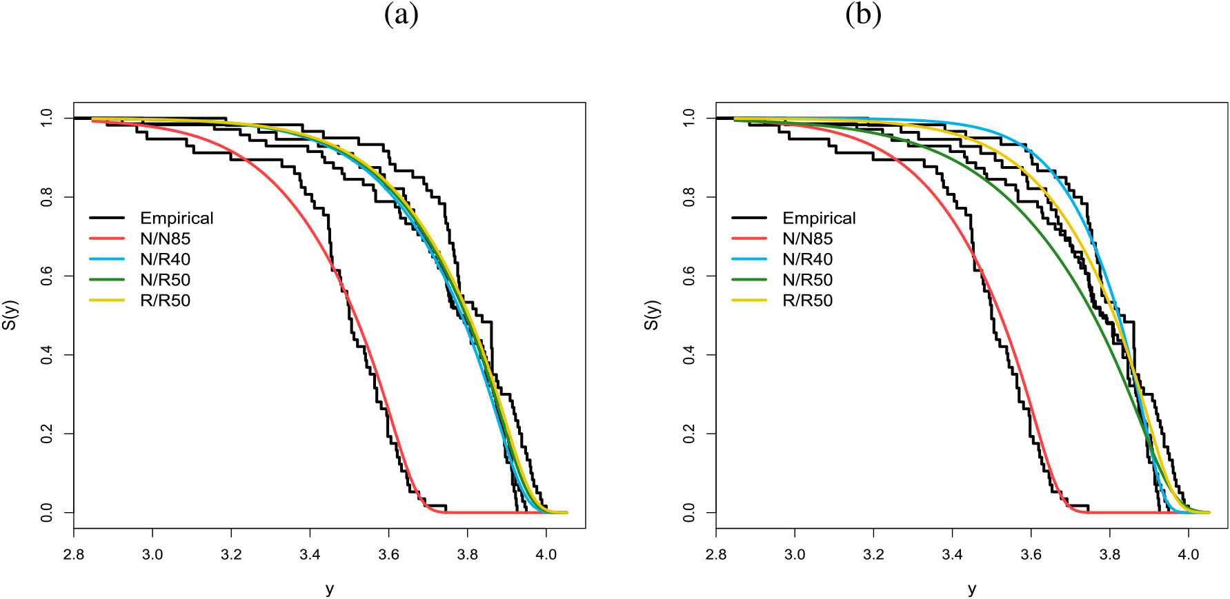 Figure 9
Estimated survival considering the log-odd log-logistic geometric Weibull (LOLLG-W) regression model for the life expectancy data. (a) Regression model with constant variance. (b) Regression model with varying dispersion.
8. CONCLUDING REMARKS
The odd log-logistic geometric-
CONFLICT OF INTEREST
There are no conflicts of interest.
AUTHORS' CONTRIBUTIONS
- –
Maria do Carmo S. Lima and Gauss M. Cordeiro contributed to the definition and properties of the new distribution.
- –
Fábio Prataviera and Edwin M. M. Ortega contributed to the regression model and applications
Funding Statement
I declare that there is no funding for this research.
ACKNOWLEDGMENTS
The financial support from CAPES and CNPq is gratefully acknowledged.
REFERENCES
Cite this article
TY  - JOUR
AU  - Maria do Carmo S. Lima
AU  - Fábio Prataviera
AU  - Edwin M. M. Ortega
AU  - Gauss M. Cordeiro
PY  - 2019
DA  - 2019/09/03
TI  - The Odd Log-Logistic Geometric Family with Applications in Regression Models with Varying Dispersion
JO  - Journal of Statistical Theory and Applications
SP  - 278
EP  - 294
VL  - 18
IS  - 3
SN  - 2214-1766
UR  - https://doi.org/10.2991/jsta.d.190818.003
DO  - 10.2991/jsta.d.190818.003
ID  - Lima2019
ER  -