
On Partially Linear Single-Index Models with Missing Response and Error-in-Variable Predictors
- DOI
- 10.2991/jsta.d.190306.006How to use a DOI?
- Abstract
In this paper, we consider a partially linear single-index model when missing responses and nonlinear regressors with measurement error are taken into account. Utilizing data imputation for missing values and regression calibration for error-prone regressors, we not only estimate the parameters in the linear part as well as the single-index part, but also estimate the nonparametric link function by local linear fit. Under normalization, all the proposed estimators for the regression coefficients and the link function are proven to be asymptotically normal, and some illustrative simulations are provided to justify our methods.
- Copyright
- © 2019 The Authors. Published by Atlantis Press SARL.
- Open Access
- This is an open access article distributed under the CC BY-NC 4.0 license (http://creativecommons.org/licenses/by-nc/4.0/).
1. INTRODUCTION
To avoid the so called “curse of dimensionality” in the nonparametric or semiparametric regression analysis, partially linear single-index models (PLSIM) emerged as an effective device for dimension reduction; see, for example, Härdle and Stoker [1], Powell et al. [2], Newey and Stoker [3], Ichimura [4], Carroll et al. [5], Xia and Härdle [6], Lu and Cheng [7], and many others. Served as an effective way of modelling a nonlinear relationship between several covariates and their response, PLSIM, however, might obtain biased estimations when the covariates and/or their response are not complete.
When one collects data (e.g., survival data), due to many practical problems, he may obtain an incomplete data set which, to such an extent, may lead to a biased estimation. Therefore, the augmentation of the missing data becomes more and more important in the data demanded world. In general, missing data might emerge in both of the responses and covariates, while in this paper we will mainly focus on the case when solely the response is missing. According to the nature of missing data, Little and Rubin [8] firstly classified the types of missingness into three categories—missing completely at random (MCAR), missing at random (MAR), and missing not at random (MNAR). In the present paper, we will consider the MAR mechanism (see, e.g., Wang et al. [9], Yun et al. [10]) which kicks in when the probability that a response is missing dose not depend on the unobserved measurements. A very important type of missingness is censoring; in particular, for the censoring case in PLSIM, Lu and Cheng [7] adopted a Kaplan–Meier-like transformation to overcome the biasedness of the estimation of the coefficients and link function. Besides, Cheng et al. [11] considers a more difficult problem concerning the estimation of the parameters and nonparametric function for a PLSIM with censored response and covariates having measurement error. However, for general missingness of the responses in PLSIM, there’s not a paper studying on it.
Another important issue concerning incomplete data is about measurement error. Measurement error models have been largely studied in the literature, for example, Fuller [12], Carroll [13], Carroll and Stefanski [14], Carroll and Li [15], Lue [16], and Fan and Troung [17], among others. It was indicated by Carroll et al. [18] that, there are three effects caused by measurement errors: first, it causes bias in parameter estimation for statistical models; second, it leads to a loss of power, sometimes profound, for detecting interesting relationship among variables; finally, it makes the features of the data, making graphical model analysis difficult. Especially, the effects of biasedness of the parameters become severer especially when the relationship between the covariates and responses appear to be nonlinear.
In this paper, we consider the following PLSIM
Among the wide variety of procedures to handle missing data, data imputation is an important step. By imputing a plausible value for each missing datum, under mild conditions, the problem can be dealt with as if they were complete. Different categories of imputations can be found in Schulte Nordholt [19]. The first classification, roughly speaking, comprises the deterministic as well as the stochastic imputations [20]. The second classification is a distinction between naive and principled approaches. The naive imputations, mainly based on analyzing complete cases (listwise or pairwise), are a quick option. For example, the imputation of an unconditional mean is a naive approach. It might lead to a biased estimate even if the data are randomly missing. Little and Rubin ([8] Chapter 3) indicated that the obvious corrections of this biasedness will obtain the same estimates as found with available case procedures. The principled approaches adopt models for both the observed and missing data on which the imputations are based.
Besides, there is a distinction between imputations according to “explicit” and “implicit” models [21, 22]. Examples can be referred to the hot-deck procedures [23], in which missing values are imputed with donor cases from the set of completely observed cases. There are still many other imputation methods, for example, linear regression imputation [24], multiple imputation [20, 25], nonparametric kernel regression imputation[26, 27]), nearest neighbor imputation [28], ratio imputation [29], regression calibration [30], and semiparametric regression imputation [9], and so on. Wang and Sun [31] adopted semiparametric imputation, semiparametric regression surrogate and inverse marginal probability weighted (IMPW) approaches, separately, to estimate
2. PROCEDURES OF ESTIMATIONS
2.1. Carroll and Li’s Transformation
As mentioned in the introduction, how to calibrate the contaminated regressors to be unbiased is a very important issue. The Carroll and Li’s [15] transformation, as stated in the following, is nothing more than a simple linear prediction of
Suppose on the other hand that, we have a replicated data rather than a validation sample. As in Carroll and Li [15] and Lue [16], we consider an important special case when
If
With this choice of
2.2. Estimations of PLSIM with Missing Response and Error-Prone Predictors
Consider the PLSIM model defined by Eq. (1). In this section, we assume that we are given a data set with partially missing response and error-prone regressors in the nonlinear single-index term. In order to remedy the biasedness of estimations caused by missing and measurement error, we propose a modified quasi log-likelihood estimation procedure via an iterative minimization algorithm.
Let
In the case when the data consists of MAR response variables and error-prone regressors, some auxiliary treatment of the data set is necessary. A difficulty common to single-index model is that, minimizing Eq. (6) involves the estimation of the nonparametric function
We denote the transformed
In order to claim that, when we replace
Now we return to the case as
Our estimation algorithm consists of the following steps:
Step 1: Treat the synthetic data
Step 2: Find
Step 3: Update
with respect toStep 4: Iterate Steps 2 and 3 until convergence is achieved.
3. ASYMPTOTIC THEOREMS FOR THE ESTIMATORS
In this section, we will establish the asymptotic normality of the estimators of the parameters emerging in the PLSIM model. Condition A is given to ensure the asymptotic properties of the estimators to hold.
Condition A.
The kernel
The random vectors
The marginal density
The random vector
The functions
For a given
Let
both
Theorem 1.
Under Condition A and the following conditions on the bandwidth:
Theorem 2.
Under the same conditions as given in Theorem 1, the estimator
It is interesting to note that
By the root-n consistency of
Theorem 3.
Let
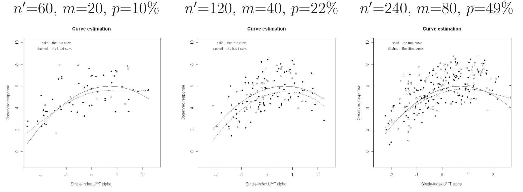
4. SIMULATION
Example
In this example, we conduct some Monte Carlo simulations to estimate the regression coefficients for an partially single-index model with incomplete data, and
Case 1:
Case 2:
Case 3:
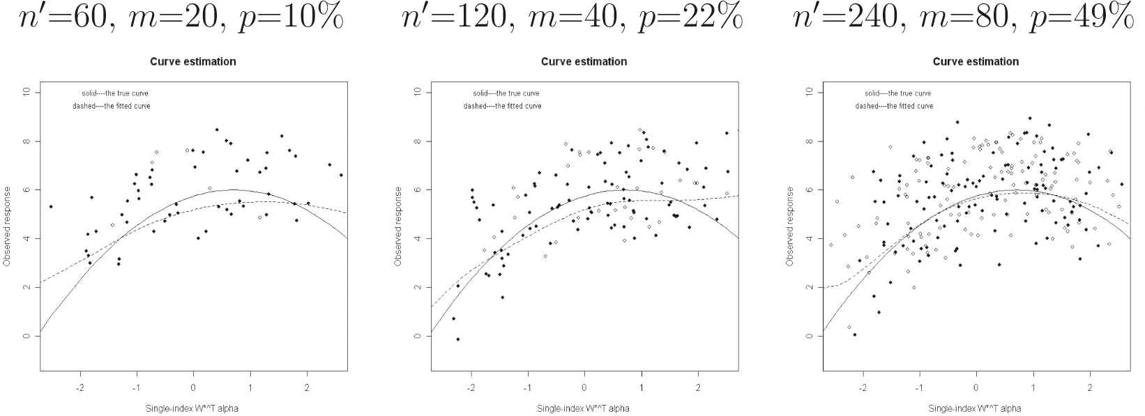
By conducting Monte Carlo simulations, the mean response rates of the above three cases are
In Table A.1 (resp. Table A.4), we report the results of
From Tables A.1 and A.4, all the proposed estimates of
APPENDIX I
Proof of Theorem 1. and 2.
The proof of Theorem 2 is just a part of arguments used in the proof of Theorem 1, therefore we omit it. Here, we give a detailed proof of Theorem 1 only.
Denote
The proof consists of two steps. The first step is to obtain an expansion for
We will show that
Denote the
Then, we will obtain the following representation:
Proof of (A.2).
Let
Solving the above equation for
Let
Since
Substituting the kernel terms in the linearized Eq. (A.4) by their asymptotic counterparts, we obtain Eq. (A.2).
Proof of (A.3).
By a Taylor expansion, we have
With
Let
By Taylor expansion, we obtain
Since
By Eq. (A.8), we get
Plugging this into Eq. (A.9) gives
This leads to
Note that by using matrix notation,
Then from Eq. (A.2) and the definition of
It is easy to see that the sixth term is Eq. (A.10) is
From
Multiplying both sides by
Section I.1. Proofs of (A.5) and (A.7)
Proof of (A.5).
Let
Equation (A.12) will be used in the proof of Eq. (A.6). First, we assume that Eq. (A.13) holds and we prove Eq. (A.12). Let
Now we prove Eq. (A.13). Let
We consider
To finish the proof, it suffices to show
We prove Eq. (A.16) but Eq. (A.17), since Eq. (A.17) is very easy to prove. We consider a more general case where
When
Suppose that
By Condition A(ii), there exists some constants
Therefore,
Similarly,
Taking
Since
This implies
Combining Eqs. (A.20) and (A.21) proves Eq. (A.18).
Now we prove Eq. (A.19). By Conditions A,
Proof of (A.7).
Since
Section I.2. Proof of (A.6)
Proof of (A.6).
Since
The proof of Eq. (A.23) is similar to that of Eq. (A.12), we omit it. Now we prove Eq. (A.24). Note that
By decomposition, it suffices to show
We shall apply the similar techniques used in the proof of Eq. (A.16) to prove the preceding three equalities. By Conditions A(ii) and (iv),
Section I.3. Proof of (A.11)
Proof of Eq. (A.11).
To prove Eq. (A.11) is equivalent to prove the following equality:
Noting that
It implies that
Now we return to the proof of Theorem 1. In Eq. (A.3),
Therefore, by Eq. (A.31), we have shown that
APPENDIX II
| MEAN | SD | RMSE | MED | MEAN | SD | RMSE | MED | ||
|---|---|---|---|---|---|---|---|---|---|
| p = 10%, n = 60 | |||||||||
| 0.707 | 0.710 | 0.061 | 0.061 | 0.707 | −1 | −0.998 | 0.148 | 0.147 | −0.999 |
| 0.707 | 0.699 | 0.064 | 0.065 | 0.707 | 2 | 2.003 | 0.149 | 0.148 | 2.007 |
| p = 22%, n = 120 | |||||||||
| 0.707 | 0.709 | 0.044 | 0.044 | 0.707 | −1 | −0.995 | 0.107 | 0.107 | −0.994 |
| 0.707 | 0.703 | 0.045 | 0.045 | 0.707 | 2 | 2.005 | 0.114 | 0.114 | 2.005 |
| p = 49%, n = 240 | |||||||||
| 0.707 | 0.704 | 0.038 | 0.038 | 0.707 | −1 | −1.002 | 0.096 | 0.096 | −0.998 |
| 0.707 | 0.708 | 0.037 | 0.037 | 0.707 | 2 | 2.006 | 0.095 | 0.095 | 2.003 |
MED, median; SD, standard derivation ; RMSE, root-mean-square error.
Descriptive statistics of
| MEAN | SD | RMSE | MED | MEAN | SD | RMSE | MED | ||
|---|---|---|---|---|---|---|---|---|---|
| p = 10%, |
|||||||||
| 0.707 | 0.686 | 0.165 | 0.166 | 0.707 | −1 | −0.992 | 0.202 | 0.202 | −1.009 |
| 0.707 | 0.682 | 0.192 | 0.193 | 0.707 | 2 | 2.011 | 0.194 | 0.194 | 2.011 |
| p = 22%, |
|||||||||
| 0.707 | 0.673 | 0.127 | 0.131 | 0.707 | −1 | −0.995 | 0.152 | 0.152 | −0.989 |
| 0.707 | 0.718 | 0.122 | 0.122 | 0.707 | 2 | 2.007 | 0.149 | 0.149 | 2.014 |
| p = 49%, |
|||||||||
| 0.707 | 0.665 | 0.105 | 0.113 | 0.695 | −1 | −1.005 | 0.137 | 0.136 | −1.001 |
| 0.707 | 0.733 | 0.095 | 0.098 | 0.719 | 2 | 1.993 | 0.127 | 0.127 | 1.993 |
MED, median; SD, standard derivation ; RMSE, root-mean-square error.
Descriptive statistics of
| MEAN | SD | RMSE | MED | MEAN | SD | RMSE | MED | ||
|---|---|---|---|---|---|---|---|---|---|
| p = 10%, |
|||||||||
| 0.707 | 0.741 | 0.105 | 0.110 | 0.715 | −1 | −1.000 | 0.206 | 0.205 | −1.003 |
| 0.707 | 0.651 | 0.129 | 0.140 | 0.699 | 2 | 1.973 | 0.203 | 0.204 | 1.964 |
| p = 22%, |
|||||||||
| 0.707 | 0.747 | 0.080 | 0.089 | 0.740 | −1 | −0.977 | 0.138 | 0.140 | −0.981 |
| 0.707 | 0.653 | 0.097 | 0.111 | 0.673 | 2 | 1.995 | 0.150 | 0.150 | 1.987 |
| p = 49%, |
|||||||||
| 0.707 | 0.752 | 0.065 | 0.079 | 0.748 | −1 | −1.017 | 0.127 | 0.128 | −1.014 |
| 0.707 | 0.651 | 0.077 | 0.095 | 0.663 | 2 | 1.984 | 0.127 | 0.128 | 1.985 |
MED, median; SD, standard derivation ; RMSE, root-mean-square error.
Descriptive statistics of
| MEAN | SD | RMSE | MED | MEAN | SD | RMSE | MED | ||
|---|---|---|---|---|---|---|---|---|---|
| p = 10%, n = 60 | |||||||||
| 0.707 | 0.709 | 0.046 | 0.046 | 0.707 | −1 | −1.002 | 0.144 | 0.144 | −1.004 |
| 0.707 | 0.702 | 0.049 | 0.049 | 0.707 | 2 | 1.992 | 0.151 | 0.151 | 1.985 |
| p = 22%, n = 120 | |||||||||
| 0.707 | 0.710 | 0.040 | 0.040 | 0.707 | −1 | −0.989 | 0.108 | 0.108 | −0.992 |
| 0.707 | 0.701 | 0.042 | 0.042 | 0.707 | 2 | 2.000 | 0.102 | 0.102 | 1.996 |
| p = 49%, n = 240 | |||||||||
| 0.707 | 0.710 | 0.038 | 0.039 | 0.707 | −1 | −0.994 | 0.097 | 0.097 | −0.988 |
| 0.707 | 0.702 | 0.041 | 0.041 | 0.707 | 2 | 2.004 | 0.092 | 0.092 | 2.005 |
MED, median; SD, standard derivation ; RMSE, root-mean-square error.
Descriptive statistics of
| MEAN | SD | RMSE | MED | MEAN | SD | RMSE | MED | ||
|---|---|---|---|---|---|---|---|---|---|
| p = 10%, |
|||||||||
| 0.707 | 0.696 | 0.136 | 0.136 | 0.707 | −1 | −1.005 | 0.230 | 0.230 | −0.985 |
| 0.707 | 0.689 | 0.151 | 0.151 | 0.707 | 2 | 2.002 | 0.183 | 0.183 | 2.003 |
| p = 22%, |
|||||||||
| 0.707 | 0.672 | 0.113 | 0.118 | 0.707 | −1 | −1.008 | 0.168 | 0.168 | −1.001 |
| 0.707 | 0.724 | 0.109 | 0.110 | 0.707 | 2 | 1.999 | 0.154 | 0.154 | 2.002 |
| p = 49%, |
|||||||||
| 0.707 | 0.675 | 0.105 | 0.109 | 0.707 | −1 | −1.014 | 0.129 | 0.130 | −1.019 |
| 0.707 | 0.724 | 0.102 | 0.103 | 0.707 | 2 | 1.988 | 0.133 | 0.133 | 1.995 |
MED, median; SD, standard derivation ; RMSE, root-mean-square error.
Descriptive statistics of
| MEAN | SD | RMSE | MED | MEAN | SD | RMSE | MED | ||
|---|---|---|---|---|---|---|---|---|---|
| p = 10%, |
|||||||||
| 0.707 | 0.748 | 0.095 | 0.104 | 0.729 | −1 | −0.977 | 0.195 | 0.196 | −0.965 |
| 0.707 | 0.645 | 0.125 | 0.140 | 0.684 | 2 | 2.021 | 0.210 | 0.210 | 2.021 |
| p = 22%, |
|||||||||
| 0.707 | 0.751 | 0.070 | 0.083 | 0.738 | −1 | −1.001 | 0.147 | 0.146 | −0.998 |
| 0.707 | 0.651 | 0.087 | 0.103 | 0.674 | 2 | 2.008 | 0.161 | 0.161 | 2.011 |
| p = 49%, |
|||||||||
| 0.707 | 0.754 | 0.073 | 0.087 | 0.750 | −1 | −1.013 | 0.136 | 0.137 | −1.016 |
| 0.707 | 0.647 | 0.087 | 0.106 | 0.661 | 2 | 1.984 | 0.134 | 0.135 | 1.996 |
MED, median; SD, standard derivation ; RMSE, root-mean-square error.
Descriptive statistics of
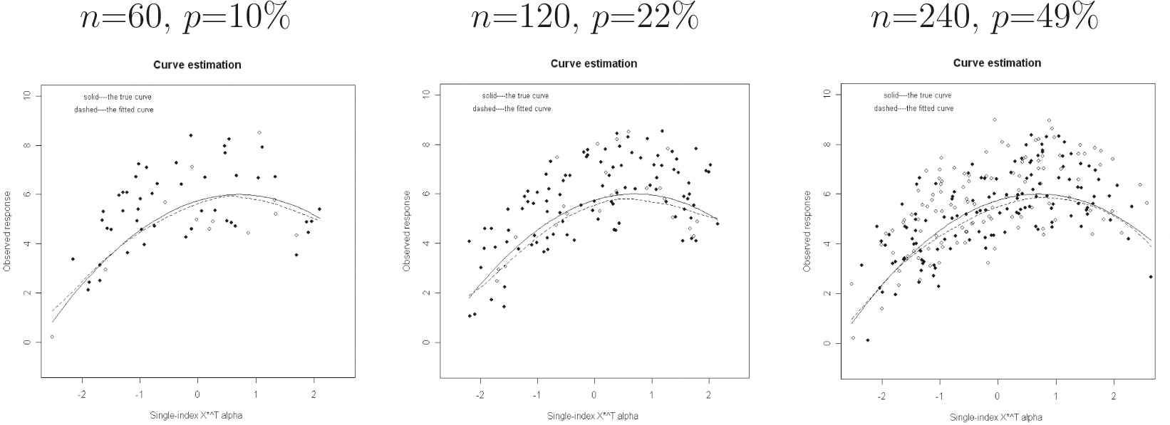
Simulated curves of
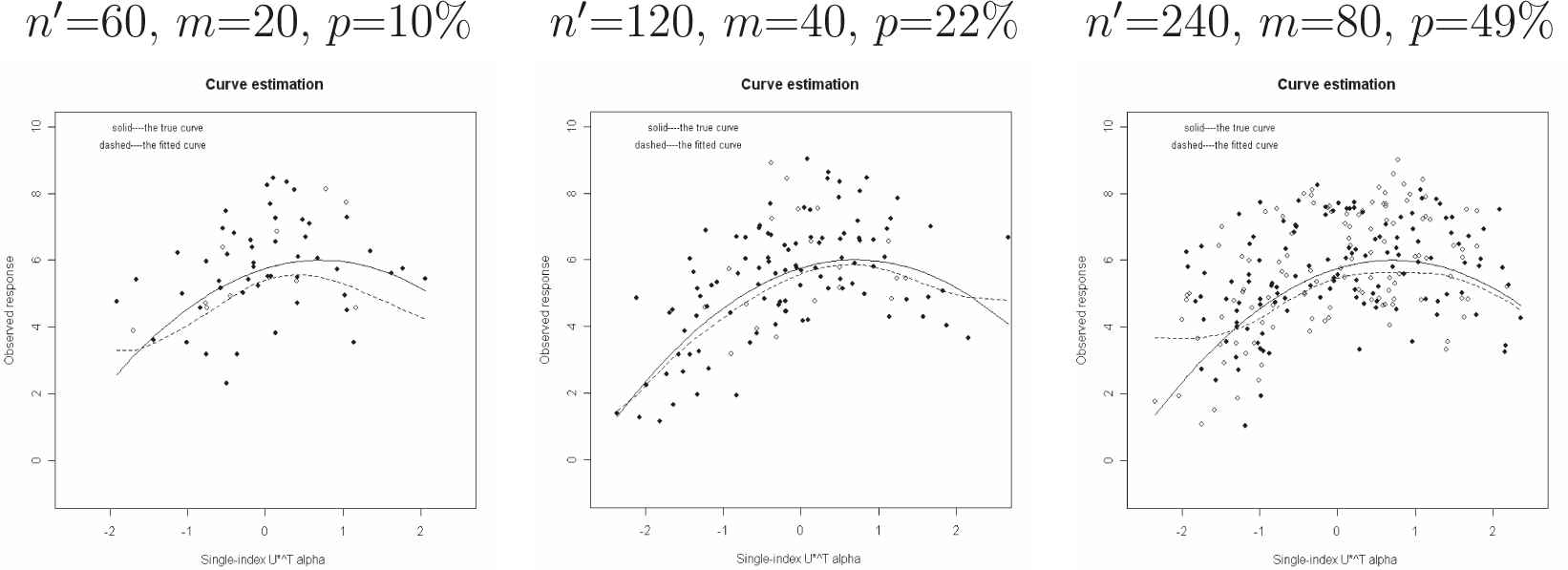
Simulated curves of
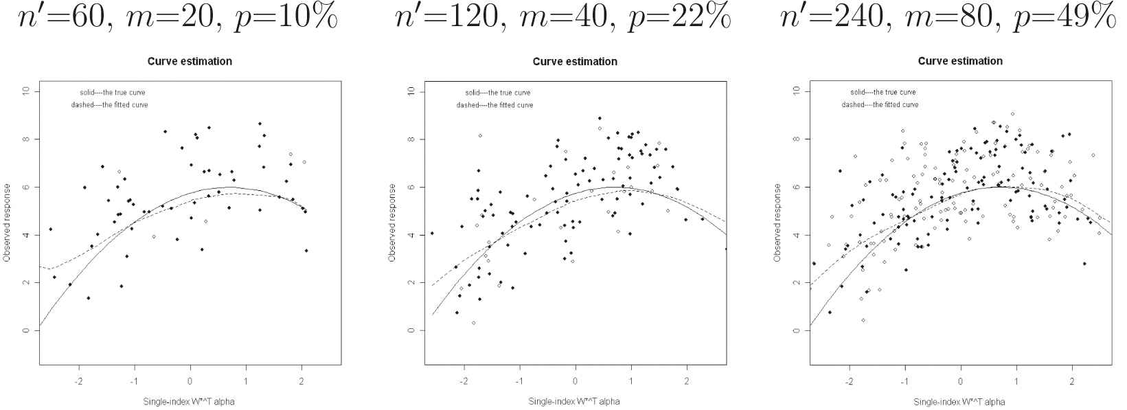
Simulated curves of

Simulated curves of
Simulated curves of
Simulated curves of
REFERENCES
Cite this article
TY  - JOUR
AU  - Tsung-Lin Cheng
AU  - Yin-Ying Lin
AU  - Xuewen Lu
AU  - Radhey Singh
PY  - 2019
DA  - 2019/04/22
TI  - On Partially Linear Single-Index Models with Missing Response and Error-in-Variable Predictors
JO  - Journal of Statistical Theory and Applications
SP  - 46
EP  - 64
VL  - 18
IS  - 1
SN  - 2214-1766
UR  - https://doi.org/10.2991/jsta.d.190306.006
DO  - 10.2991/jsta.d.190306.006
ID  - Cheng2019
ER  -