1. Introduction

Optimal impulsive rendezvous is aimed at obtaining minimum-fuel guidance strategy for spacecraft rendezvous, which has attracted considerable attention. Despite that Lawden’s necessary conditions¹ for optimal impulsive trajectories and Lion’s improving methods² for non-optimal trajectories have provided some guidelines to solve the optimal problem where the initial states and rendezvous time are specified, the distributions of optimal models cannot be obtained clearly in these way. So far, only Prussing’s theory³ of optimal impulsive rendezvous on close circular orbits is complete in its theoretical system, which derives the solutions and distributions of optimal impulsive models by solving the primer vector equations and boundary value problem. A reference frame in mean velocity orbit was built by Frank⁴, and showed better performance in describing the impulse locations and magnitudes than the mean radius orbit in Prussing’s results. Xie⁵ focused on the selection of reference frame for optimal impulsive rendezvous, and investigated the effect on the classification, distribution and guidance precision. For the case of elliptic orbit rendezvous, Wang⁶ used the state transition matrix given by Yamanaka⁷ to calculate the optimal solution of four-impulse model, but the analytical solution and the distribution are difficult to be achieved. Chen^8,9 studied the ellipse-to-circle coplanar rendezvous based on his results on the dynamical equations for elliptic orbit rendezvous in low eccentricity, and provided the solutions and distributions of all types optimal models. Motivated by which, our previous work¹⁰ considered the ellipse-to-ellipse coplanar rendezvous and obtained the analytical solution and distribution of four-impulse model. In this paper, we will further investigate the Hohmann-type model for optimal impulsive ellipse-to-ellipse coplanar rendezvous.

2. Dynamics Description

The relative motion between two spacecrafts in elliptic orbits was derived in our previous work¹⁰, which is still used in this paper and given as follow:

The initial and terminal states of system (1) are

The states at phase angle τ was also deduced[10]:

3. Optimal Hohmann-Type Rendezvous

The solution to primer vector equations corresponding to system (1) can be given in the following form:

3.2. Distribution of Hohmann-type model

The distribution of optimal Hohmann-type rendezvous is to illustrate the existence of feasible solution. To investigate the distribution, rendezvous time is chosen as the X-coordinate and the special phase angle defined below as Y-coordinate:

(16)δθF=−β+1.5d4τF−d3sin(τF+φ)+d3sinφ

Let τ_Fh be rendezvous time solved by (11) and (14), and δθ_Fh is the corresponding special phase angle. If τ_F = τ_Fh and δθ_F = δθ_Fh, then it is just the Hohmann transfer. The two impulses are implemented at τ₁ = 0 and τ₂ = τ_F. However, when the real rendezvous time is longer than τ_Fh, the coasts are needed to save the fuel.

If τ_F > τ_Fh and δθ_F = δθ_Fh, it is a Hohmann model with terminal coast. The two impulses are implemented at τ₁ = 0 and τ₂ = τ_Fh, and the residual time τ_F – τ_Fh is for terminal coast. The special phase angle δθ_F and rendezvous time τ_F should satisfy the following relation

(17)δθF=δθFh+1.5d4(τF−τFh)         +d3sin(τFh+φ)−d3sin(τF+φ)τFh=τ2−τ1,τF∈[τFh,+∞)

If τ_F > τ_Fh and the special phase angle δθ_F satisfies

(18)δθF=δθFh−1.5d4(τF−τFh)         +d3sin(τF−τFh+φ)−d3sinφτFh=τ2−τ1,τF∈[τFh,+∞)

then, after the initial coast for time τ_F – τ_Fh, the special phase angle will become exactly δθ_Fh. This case is a Hohmann model with initial coast, and the impulses are implemented at τ₁ = τ_F – τ_Fh and τ₂ = τ_F.

Let

(19)δθFh1=δθFh+1.5d4(τF−τFh)+d3sin(τFh+φ)−d3sin(τF+φ)δθFh2=δθFh−1.5d4(τF−τFh)+d3sin(τF−τFh+φ)−d3sinφ

If τ_F > τ_Fh and δθ_Fh1 < δθ_F < δθ_Fh2, then there exists a Hohmann model with both initial coast and terminal coast. As shown in Fig. 1., this case is illustrated in the middle of the curves expressed by (17) and (18), that is the shadow part. Denote (τ_F0, δθ_F0) as the intersection point of the curves determined by (16) and (18), then the two impulses are implemented at τ₁ = τ_F0 – τ_Fh and τ₂ = τ_F0. The initial and terminal coast last for time τ_F0 – τ_Fh and τ_F – τ_F0, respectively.

Fig 1

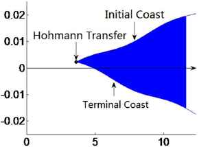
Distribution of Hohmann-type model

From the above, the optimal Hohmann-type impulsive rendezvous has four models, all of whose impulse magnitudes are determined by (9) and (15), and impulse direction is along the tangential direction.

4. Simulations

In this section, simulation examples are presented to show the guidance performance and distribution of Hohamman-type impulsive rendezvous.

4.2. Distribution of Hohmann-type model

To investigate the distribution of Hohmann-type ellipse-to-ellipse rendezvous, we take rendezvous time τ_F as the X-coordinate and δθ_F/d₄ as Y-coordinate. Fig. 2 shows the distribution of Hohmann-type model with different true anomalies and eccentricities.

Fig 2

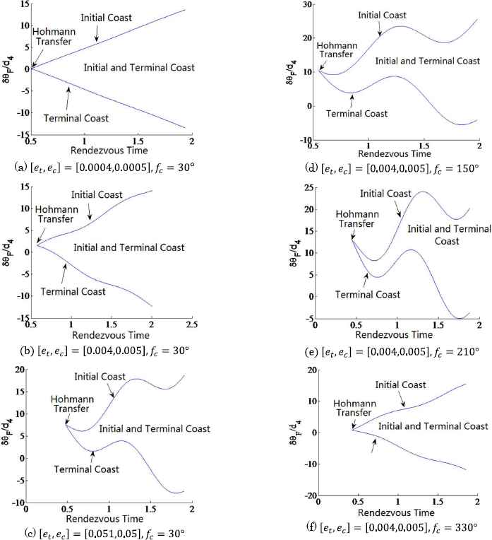
Distributions with different true anomalies and eccentricities

5. Conclusion

This paper extends our previous work¹⁰ to the Hohmann-type optimal impulsive rendezvous. By defining the special phase angle, we derived the analytical solution for Hohmann transfer, and obtained that the optimal Hohmann-type impulsive rendezvous has four models, i.e. Hohmann transfer, Hohmann with initial coast, Hohmann with terminal coast and Hohmann with both coasts. In further research, we will integrate all optimal models in one map, including four-impulse, three-impulse, three-impulse with coasts, two- impulse, two-impulse with coasts, and Hohmann-type.

Acknowledgements

This work was supported by NSFC (61327807, 61521091, 61520106010, 61134005) and the National Basic Research Program of China (973 Program: 2012CB821200, 2012CB821201)