1. INTRODUCTION

Solid waste is inextricably related to industrial growth and urbanization. Countries’ economic prosperity rises as they urbanize. Consumption of goods and services rises in tandem with the levels of life and disposable incomes, resulting in an increase in waste generation. According to Karak et al. [1], nearly 1.3 billion tons of Municipal Solid Waste (MSW) are produced globally per year, or 1.2 kg each capita per day. The real per capita figures, on the other hand, are extremely volatile, as waste generation rates vary greatly across nations, cities, and also within cities. Solid waste is traditionally thought of as a ‘urban’ epidemic. Rural people, on average, are wealthier, consume less store-bought goods, and reuse and recycle more. As a result, waste production rates in rural areas are much smaller. More than half of the world’s population now lives in cities, and the pace of urbanization is rapidly growing. By 2050 [2], as many people will live in cities as the population of the whole world in 2000. This will add challenges to waste disposal. People and companies would almost definitely have to take on greater responsibility for waste generation and disposal, especially in terms of product design and waste separation. A stronger focus on ‘urban extraction’ is also expected to arise, as cities are the largest supplier of resources like metal and paper. Tons of waste are created every day, creating a major problem for various cities and municipal authorities due to a lack of landfill capacity to dispose of such waste. Toxic hazard materials in the waste cause health concerns as well as environmental harm. Due to a lack of landfill space and environmental pollution, as well as its economic effects, recycling has become a major problem [3].

The methods from neural networks [4] and other classification methods [5], tree classifier, and quadratic discriminant analysis [3], with optical sensors and controller [6], with image processing software capability [7,8] can provide a promising results for paper and plastic sorting for waste management using artificial intelligence. Hence, for many artificial intelligence methods, the optimized features need to be identified, to ensure correct classification of the mixed waste.

Many interests among researchers published on classification accuracy which discussed on best feature selection [9–11]. Still, to some researchers, the focus also arises on classification accuracy and computational time [12,13]. However, the scope of this work is to show how the reduction of features can contribute to higher classification accuracy of mixed waste classification.

2. MATERIALS AND METHODS

2.1. Dataset and Training

In this study, 320 sample images were taken for seven different dry waste garbage classes. The features data was extracted from greyscale, segmented greyscale images and binarized image of the captured RGB images using Matlab2019b. Table 1 dataset used for training in each class.

Type of mixed waste	Dataset
Bottle	40
Cup	50
Plastic box	40
Paper box	40
Crumble paper/plastic	50
Flat paper/plastic	50
Tin can	50
Total dataset	320

Table 1

Dataset of classes

2.1.1. Features extraction

From the observation of mixed waste classes which consist of crumble (paper/plastic), flat (paper/plastic), tin can, bottle (plastic/glass), cup (paper/plastic), plastic box and paper box, the following 40 features have been selected for the class of interest as shown in Table 2 which extracted from Figure 1 via image processing method.

Features	Source image	Formula
F1: Round measure of sample images	Greyscale of segmented sample image (Figure 1)	4πA/P2 (1) where, A is the area of the image, P is the perimeter of the image
F2: Mid-point symmetry	Computation of white pixel summation array C. (a) Segmentation filter. (b) Graph of white pixel summation array C (Figure 2)	o ∑y=1na(y)=1∑z=1nb(z) *100 (2) where o is the total number of elements and y is the corresponding number of elements of array a, z is the corresponding elements of array b.
		Array a is the first half of the array C, and array b is the second half of the array C.
F3: Skewness	Computation of white pixel summation array C. (a) Segmentation filter. (b) Graph of white pixel summation array C (Figure 2)	E(C−µ)3σ3 (3) where C is the white pixel summation array, E is the expected value of quantity, μ is the mean of C, σ is the standard deviation of C.
F4: Mode	Computation of white pixel summation array C. (a) Segmentation filter. (b) Graph of white pixel summation array C (Figure 2)	It returns the mode of C, which is the most frequently occurring value in C. When there are multiple values occurring equally frequently, mode returns the smallest of those values.
F5: Kurtosis	Computation of white pixel summation array C. (a) Segmentation filter. (b) Graph of white pixel summation array C (Figure 2)	E(C− µ)4σ4 (4) where C is the white pixel array, E is the expected value of quantity, μ is the mean of C, σ is the standard deviation of C.
F6: Mean	Computation of white pixel summation array C. (a) Segmentation filter. (b) Graph of white pixel summation array C (Figure 2)	1N∑i=1NCi (5) where C is the white pixel array, N is the observations/values in the array.
F7: Standard deviation	Computation of white pixel summation array C. (a) Segmentation filter. (b) Graph of white pixel summation array C (Figure 2)	1N−1∑i=1N|Ci−μ|2 (6) where C is metric of the white pixel summation of the image with N number of values greater than 0, and μ is the mean of C.
F8: Zero-scores	Computation of white pixel summation array C. (a) Segmentation filter. (b) Graph of white pixel summation array C (Figure 2)	n[|x−µσ|>2] (7) where n is the total numbers of absolute value array, μ is the mean and σ is the standard deviation of the C.
F9: Quantile	Computation of white pixel summation array C. (a) Segmentation filter. (b) Graph of white pixel summation array C (Figure 2)	max(quantile(C,p)) (8) where p = 25
F10: Derivative variance	Computation of white pixel summation array C. (a) Segmentation filter. (b) Graph of white pixel summation array C (Figure 2)	1N−1∑i=1N|Ci−µ|2 (9) where C is metric of the white pixel summations of the image with N number of values greater than 0, and μ is the mean of C.
F11: Standard deviation	Greyscale of segmented sample image (Figure 3)	1N−1∑i=1N|Ci−μ|2 (10) where C is metric of the greyscale of the segmented image with N number of values greater than 0, and μ is the mean of C.
F12: Entropy	Greyscale of segmented sample image (Figure 3)Entropy of the segmented grey image.	−sum(p.*log2(p)) (11) where p contains the normalized histogram counts.
F13: Greyscale level ratio range (>40 and <111)	Greyscale of segmented sample image (Figure 3)	Percentage of grey pixels having intensity greater than 40 and less than 111 in the segmented grey image pixel array.
F14: Greyscale level ratio range (>110 and <181)	Greyscale of segmented sample image (Figure 3)	Percentage of grey pixels having intensity greater than 110 and less than 181 in the segmented grey image pixel array.
F15: Greyscale level ratio range (>180 and <=255)	Greyscale of segmented sample image (Figure 3)	Percentage of grey pixels having intensity greater than 180 and less than or equal to 255 in the segmented grey image pixel array.
F16: Grey-level co-occurrence matrix (Contrast)	Greyscale of segmented sample image (Figure 3)	∑i,j|i−j|2p(i,j) (12) where p contains the normalized histogram counts. (i, j) are position values of pixels.
	Measure of the intensity contrast between a pixel and its neighbor over the whole image.
F17: Grey-level co-occurrence matrix (Correlation)	Greyscale of segmented sample image (Figure 3)	∑i,j (i−µi)(j−µj)(i,j)σiσj (13) where (i, j) position values of pixels. μ is the mean of the pixel at the position (i, j). σ is standard deviation of pixel at the position (i, j).
	Measure of correlated pixel to its neighbor over the whole image.
F18: Grey-level co-occurrence matrix (Energy)	Greyscale of segmented sample image (Figure 3)	∑i,jp(i,j)2 (14) where p contains the normalized histogram counts. (i, j) are position values of pixels.
	Returns the sum of squared elements in the GLCM.
F19: Grey-level co-occurrence matrix (Homogeneity)	Greyscale of segmented sample image (Figure 3)	∑i,jp(i,j)1+|i−j| (15) where p contains the normalized histogram counts. (i, j) are position values of pixels.
	Returns a value that measures the closeness of the distribution of elements in the GLCM to the GLCM diagonal.
F20: Entropy	Binarized image of segmentation filter (Figure 2a)	−sum(p.*log2(p)) (16) where p contains the normalized histogram counts.
	Entropy of binary of the segmented image of the samples.
F21–F40	Mean of Gabor filters which were created from segmented grey image, with four different frequencies f, and six different wavelengths λ.	Source image: Greyscale of segmented sample image (Figure 3)
		f = [0, 90, 135, 45]
		λ = [2.8, 5.65, 11.314, 22.63, 45.25, 90.51]

GLCM, Grey-level co-occurrence matrix.

Table 2

Features list

Figure 1

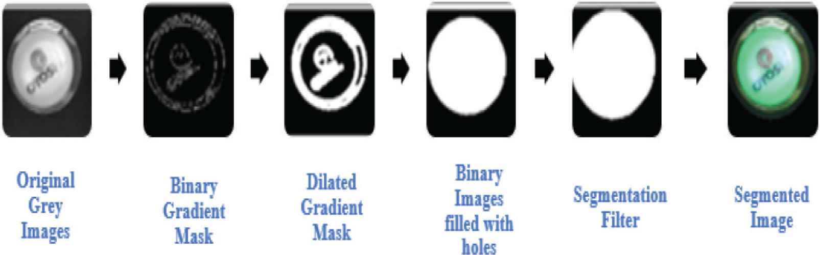
Segmentation stages for bottle class sample.

Figure 2

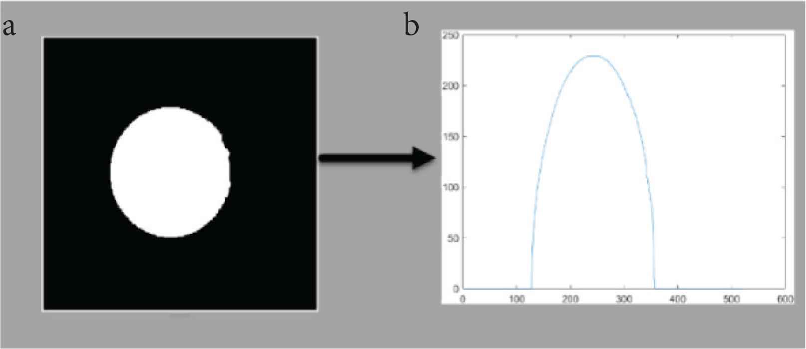
Computation of white pixel summation array C. (a) Segmentation filter. (b) Graph of white pixel summation array C

Figure 3

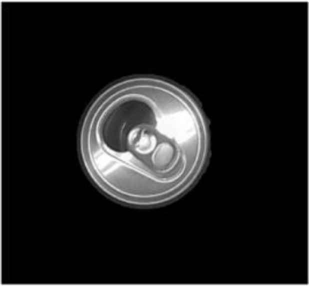
Greyscale of segmented image.

2.1.2. Classifiers used for training

Table 3 shows the types of classifiers used with respect to their specifications. Figure 4 shows the block diagram for training of the developed system.

No	Classifiers	Specifications
1	Support Vector Machine – Cubic (C.SVM)	Kernel function: Cubic, k = 1, One-vs-one method
2	Support Vector Machine – Quadratic (Q.SVM)	Kernel function: Cubic, k = 1, One-vs-one method
3	Ensemble Bagged Trees (E. Bagged Trees)	Maximum no of splits = 342, no of learners = 30, learning rate = 0.1
4	k-Nearest Neighbor (Fine.kNN)	k = 10
5	Ensemble Boosted Trees (E. Boosted Trees)	Maximum no of splits = 20, no of learners = 30, learning rate = 0.1

Table 3

Classifiers and specifications

Figure 4

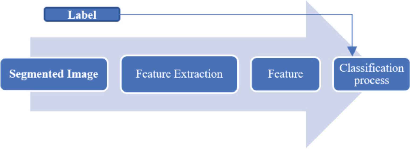
Flowchart for classifier training.

3. RESULTS AND DISCUSSION

3.1. Features Selections

There are several stages of feature selections carried out from this study. The first stage, all 40 features are used. However, accuracy of the 40 features during training was less than 77.8%. To address the shortcoming, several tests were conducted and number of redundant features which contribute less and reduced the percentage rate of the training were removed from the list.

In the second stage, 20 features were selected from the 40 features. After many features tuning and combination, it was observed that F1–F5, F7, F8, F10, F14, F30–F35, F37–F40 were insignificant and did not contribute to the classification process. These features were removed which then contributed to mean of 79.12%

In the third stage, only 17 features were used which consists of F9, F11–F13, F15–F24, F26–F28. For these 17 features, Q.SVM and C.SVM showed accuracy above 88%.

In the fourth stage, F9 and F11 were removed. F12, F13, F15–F24, F26–F28 were maintained. However, the accuracy was severely impacted with average results lest than 80%. Figure 5 summed up the performance with respect to features selections stages.

Figure 5

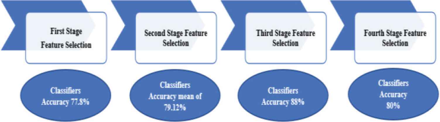
Summary of features selections with respect to each stage.

4. CONCLUSION

From this study, it was observed that relevant features and accuracy are good matched to ensure the performance of mixed waste classification. The relevant features were studied stage by stage. In the first stage, even though more features were assigned, the classifiers training showed poor performance. In the second stage, after reduction of features, by experimenting the features and training rate, the redundant features which contributed to low accuracy have been removed. Eventually the classification rate of training increased to average of 79.12%. Further reduction to 17 features, have contributed to higher average accuracy of 86.22%. However, further reduction did not contribute to better classification rate. The selected 17 features with Q.SVM as classifier also proved with higher accuracy for training with 90.69% and testing with 89.9%. In a nutshell, the important of the correct features selection is crucial for mix waste classification. Optimal features selection, proved for higher accuracy of mixed waste classification. On contrary, more features not necessarily contributed to higher accuracy.

CONFLICTS OF INTEREST

The authors declare they have no conflicts of interest.

AUTHORS INTRODUCTION

Mr. Hassan Mehmood Khan

He received his B.E. in Electronics from Dawood University of Engineering and Technology, Pakistan in 2009. He is currently submitted his Master of Engineering Science with University of Malaya, Malaysia. From 2015 to 2020, he has been as Head of Department (Mechatronics) at MIT Academy Sdn. Bhd. His research interests include automation, image processing, machine learning, and artificial intelligence.

Dr. Norrima Mokhtar

She received the B. Eng. degree in Electrical Engineering from University of Malaya in 2000. After working two years with the International Telecommunication Industry with attachment at Echo Broadband GmbH, she managed to secure a Panasonic Scholarship which required intensive screening at the national level in 2002. She finished her Master of Engineering (Oita, Japan) under financial support received from Panasonic Scholarship in 2006. Consequently, she was appointed as a lecturer to serve the Department of Electrical Engineering, University of Malaya immediately after graduating with her Master of Engineering. As part of her career development, she received a SLAB/SLAI scholarship to attain her PhD in 2012. Her research interests are signal processing and human machine interface.

Dr. Heshalini Rajagopal

She received her Master’s degree from the Department of Electrical Engineering, University of Malaya, Malaysia in 2016. She has passed her PhD Viva Voce in University of Malaya, Malaysia recently. She received the B.E. (Electrical) in 2013 and M. Eng. Sc. in 2016 from University of Malaya, Malaysia. Currently, she is a lecturer in Manipal International University, Nilai, Malaysia. Her research interest include image processing, artificial intelligence and machine learning.

Dr. Anis Salwa Mohd Khairuddin

She received PhD in computer engineering at Universiti Teknologi Malaysia (UTM). She received the B. Eng (Hons) Electrical and Electronics Engineering from Universiti Tenaga Nasional, Malaysia, in 2007 and Masters degree in computer engineering from Royal Melbourne Institute of Technology, Australia, in 2009. She is currently a Senior Lecturer from University of Malaya. Her current interests include pattern recognition, image analysis, and artificial intelligence.

Dr. Wan Amirul Bin Wan Mohd Mahiyidin

He received the M. Eng. degree from the Imperial College London in 2009, the M.Sc. degree from University of Malaya in 2012, and the PhD degree from University of Canterbury in 2016. He is currently a senior lecturer at the Department of Electrical Engineering, University of Malaya. His research interests are multiple antennas system, cooperative MIMO, channel modelling and positioning system.

Dr. Noraisyah Binti Mohamed Shah

She received the B. Eng. degree from University of Malaya in 1999, Master Degree from Oita Universitym, Japan, and the PhD degree from George Mason University. She is currently a senior lecturer at the Department of Electrical Engineering, University of Malaya. Her research interests are image processing, machine learning and satellite communication.

Prof. Dr. Raveendran Paramesran

He (SM’01) received the B.Sc. and M.Sc. degrees in electrical engineering from South Dakota State University, Brookings, SD, USA, in 1984 and 1985, respectively, and the PhD degree from the University of Tokushima, Japan, in 1994. He was a Systems Designer with Daktronics, USA. He joined the Department of Electrical Engineering, University of Malaya, Kuala Lumpur, in 1986, as a Lecturer. In 1992, he received a Ronpaku Scholarship from Japan. He was promoted to Associate Professor in 1995, then was promoted to Professor in 2003. His research areas include image and video analysis, formulation of new image descriptors for image analysis, fast computation of orthogonal moments, analysis of EEG signals, and data modeling of substance concentration acquired from non-invasive methods. His contributions can be seen in the form of journal publications, conference proceedings, chapters in books and an international patent to predict blood glucose levels using non-parametric model. He has successfully supervised to completion 14 PhD students and 12 students in M. Eng. Sc. (Masters by research). He is currently a member of the Signal Processing Society.