
Design of an Optimized GMV Controller Based on Data-Driven Approach
- DOI
- 10.2991/jrnal.k.210922.006How to use a DOI?
- Keywords
- PID controller; GMV; Nelder–Mead method; data-driven approach
- Abstract
This paper presents a data-driven scheme that can obtain the optimized Generalized Minimum Variance (GMV) control parameters by applying the Nelder–Mead (NM) method based on Proportional-Integral Derivative (PID) controller for linear system. An adjustable λ is included in the GMV-PID controller. In the existing GMV-PID controller, the PID parameters are calculated by simply changing λ manually. Therefore, it is hard to get desirable control performance. The NM method is introduced to improve the control performance. The application of NM method can optimize the calculation of λ. However, the objective function in NM method needs the output calculation. In other words, the model information is inevitably to obtain output. To achieve model-free design scheme, the estimation of closed-loop response method is introduced in database-driven approach. Using obtained closed-loop data can predict the output and then substitute it into the objective function without any model information of the process. The effectiveness is verified by experiment.
- Copyright
- © 2021 The Authors. Published by Atlantis Press International B.V.
- Open Access
- This is an open access article distributed under the CC BY-NC 4.0 license (http://creativecommons.org/licenses/by-nc/4.0/).
1. INTRODUCTION
Despite the new results in control theory that have been achieved by researchers year-by-year all over the world, the Proportional-Integral Derivative (PID) controller [1] in all control design techniques is the most popular controller used in the process industries. It has a long history in the automatic control field and can assure satisfactory performances with simple algorithm for a wide range of processes. The structure is very simple, and it is very easy to grasp the physical meaning of PID parameters. Therefore, over the last half-century, a great deal of academic and industrial effort has focused on defining PID parameters.
In recent years, some methods for calculating PID parameters have been proposed, but these methods are model-based and require system identification to calculate the PID parameters. However, it is hard to tune these parameters because most real systems generally have high-order lag factors and uncertainness. However, some data-based methods have gradually been proposed. It does not require system identification to calculate PID parameters only through closed-loop data, which greatly reduces the calculation cost.
Among the existing control strategies, using the Minimum Variance (MV) as the benchmark can claim to be successful. The basic idea behind the MV index is to only consider the controller error variance. However, few of the available techniques in use take the control effort or the manipulative variable activity into account. Then, the Generalized Minimum Variance (GMV) [2] is proposed, and it takes into account controller error variance as well as the manipulating variable variance, which can achieve model-free. In the existing GMV-PID controller [3], an adjustable parameter λ (a weighting factor penalty on the manipulating variable) is included, and the PID parameters are calculated by simply changing λ manually. Therefore, it is hard to get desirable control performance.
To improve the control performance, the Nelder–Mead (NM) method [4] is introduced. The NM method is different from the simplex algorithm in linear programming. It does not use any derivative operation and the algorithm is relatively simple. It can optimize the calculation of the most suitable parameter λ. However, the objective function in NM method needs the output calculation. In other words, the model information is inevitably to obtain output. To achieve model-free design scheme, the estimation of closed-loop response method is introduced in database-driven approach. Using obtained closed-loop data can predict the output and then substitute it into the objective function without any model information of the process. The effectiveness of the proposed scheme is verified by the experiment of tank system.
The rest of this paper is organized as follows: the problem is formulated in Section 2; the proposed scheme is the main topic in Sections 3 and 4; Section 5 provides the experiment and analysis, and Section 6 concludes the paper.
2. OVERVIEW OF THE DATA-DRIVEN GMV CONTROLLER
This paper gives the details of the proposed method which describes a design scheme for data-driven GMV-PID controller which can obtain GMV control parameters by applying the NM method and the estimation of closed-loop response based on PID controller. In Figure 1, an adjustable parameter λ is included in the GMV-PID controller, therefore PID parameters are calculated by simply changing λ. Using the method of estimation of closed-loop response to predict new output, then the application of NM method can optimize the calculation of the most suitable λ according to the predict output and get optimal PID parameters without any model of the process.

The block diagram of data-driven GMV controller.
3. GENERALIZED MINIMUM VARIANCE CONTROL
3.1. System Description
Consider the following system:
3.2. Control Design
The GMV control law for the system (1) can be derived by minimizing the following cost function:
Here, ϕ(t + k + 1) is the generalized output given by following equation:
Moreover, P(z−1) is the design polynomial and it is designed based on the following equation. Where, the order of E(z−1) and F(z−1) are set to decide these coefficients uniquely from ΔA(z−1) and P(z−1).
Here, the optimum predictive value at t is defined by
The control law is described as the following equation:
To obtain an optimum predictive value
The least-square method is applied to the obtained closed-loop data to minimize the square sum of these residual errors, then the parameters of G(z−1) and F(z−1) are identified without system parameters. The velocity type of PID control is given by the following equation:
KP, KI, and KD denotes the proportional gain, the integral gain and the derivative gain. By replacing the polynomial G(z−1) by the steady-state term G(1), the following equation can be obtained:
Therefore, PID parameters can be calculated as follows:
4. EVOLUTIONARY COMPUTATION USING NELDER-MEAD METHOD
4.1. Nelder–Mead Method
The Nelder–Mead method is briefly explained to calculate the user-specified parameter λ. Each top of the triangle is determined as Si = λi. In this paper, the objective function is determined by
- •
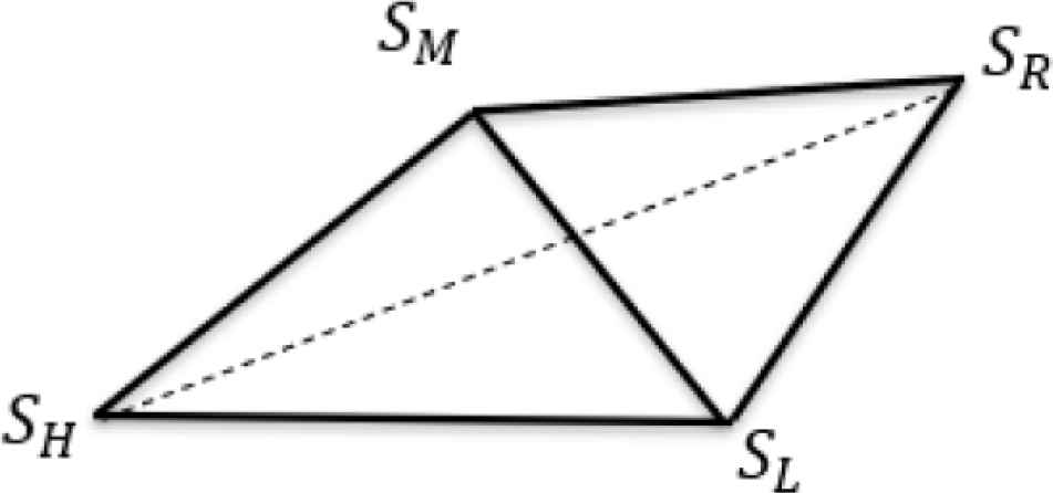
Reflection
SR is determined as SR = (1 + β)SG − βSH, where β is set as β > 0, and it corresponds to the ratio of distances SRSG and SHSG.
- •
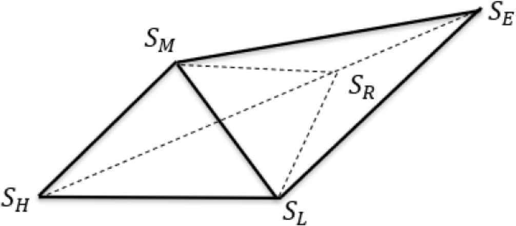
Expansion
SE is determined as SE = (1 − γ)SG + γSH, where γ is set as γ > 1, and it corresponds to the ratio of distances SESG and SRSG.
- •
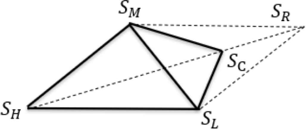
Contraction
SC is determined as SC = (1 − η)SG + ηSH, where η is set as 1 > η > 0, and it corresponds to the ratio of distances SCSG and SHSG.
- •
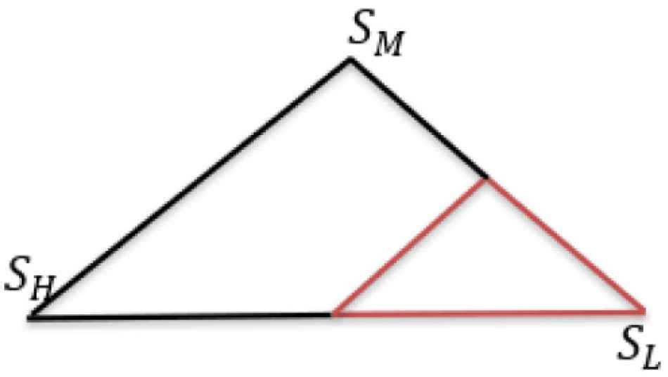
Reduction
SH and SM are moved in the direction of SL.
The proposed control system can be designed by calculate the most suitable λ by the steps based on the mentioned procedure. The proposed control system can be designed by calculating the most suitable λ by the steps based on the mentioned procedure in Figures 2–6. The above algorithm can be summarized as follows:
- 1.
Construct the initial working simplex S.
- 2.
Repeat the following steps until the termination test is satisfied. Calculate the termination test information.
- 3.
If the termination test is not satisfied, then transform the working simplex.
- 4.
Return the best vertex of the current simplex S and the associated function value.
Reflection of the Nelder–Mead method.
Expansion of the Nelder–Mead method.
The contraction of the Nelder–Mead method.
Reduction of the Nelder–Mead method.
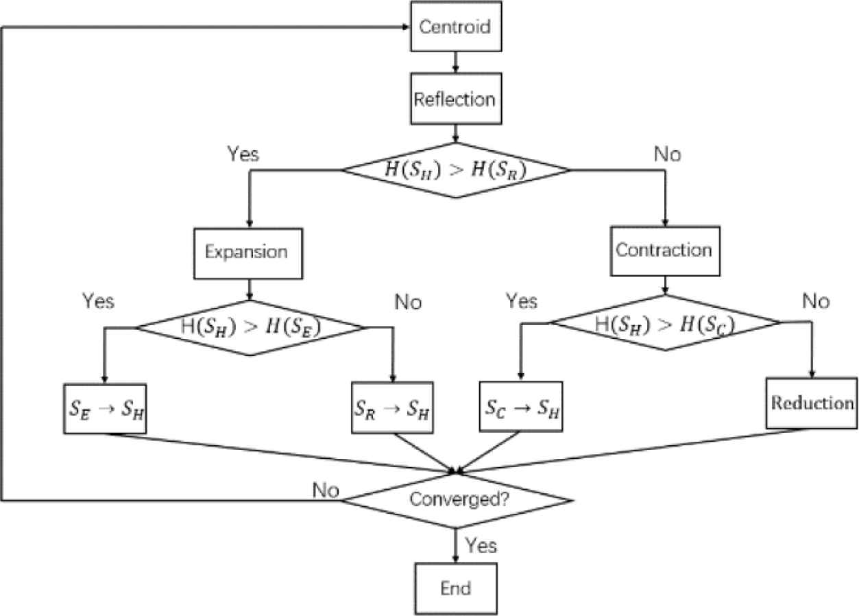
Procedure of the Nelder–Mead method.
4.2. Estimation of Closed-Loop Response
To achieve model-free design scheme, the estimation of closed-loop response method [5] is introduced in data-driven approach. Using obtained closed-loop data can predict the output and then substitute it into the objective function without any model information of the process. The estimation of closed-loop response method is used to predict the output using only the initial data without any model of the process.
The superposition principle is valid for input–output relations in Linear Time Invariant (LTI) systems. In this method, the response is predicted by describing the predicted input and output using the superposition of the input–output relations already obtained. First, we describe the prediction of the response of an arbitrary LTI system, and then we describe the prediction of the response of a closed-loop system composed of LTI systems. Response prediction for linear systems suppose that the input–output data pairs u0, y0 (t = 0, 1, …, N − 1) of an arbitrary discrete-time LTI system G are obtained. The relationship between u0, y0 is given by:
We consider predicting the response yd from u0, y0 when an arbitrary input ud given by the designer is applied to G. Where ud, yd (t = 0, 1, …, N − 1) satisfies the following equation.
Since G is an LTI system, if u0, y0 and the different input-output relations u1, y1 are known, the following relations hold for any constants κ and ι.
The relationship between both equation is commonly referred to as the superposition principle. When the data length N of ud and yd is large enough, it is difficult to determine κ and ι such that ud and yd are obtained from only two sets of input and output data. To adjust each time series, it is desirable to prepare N sets of input and output data. Therefore, it is desirable to prepare N pairs of input and output data to adjust each time series, so that u0 and y0 can be adjusted by k(k = 0, 1, 2, …, N − 1) of u0 and y0, respectively. They are then introduced in vector form as in equations.
We also define the vectors ud and yd.
If u0(0) is non-zero, then the vectors uk and yk are linearly independent for each k. Therefore, ud can be expressed using the coefficient vectors a and uk as in equation.
Here, U is regular if u0 is non-zero. Solving from the relationship, ud(0) = a0u0(0), ud(1) = a0u0(1) + a1u0(0), a, which corresponds to κ and ι, can be obtained sequentially and uniquely determined by the designer by giving ud. Using the coefficient spectrum κ obtained in this way, yd can be obtained from the superposition principle as shown in next equation.
U and Y are described by the previously obtained input and output data u0, y0. Using the known data, the output yd of system G for any input ud can be predicted.
In this paper, the pseudo reference signal is described as the following equation:
5. EXPERIMENTAL EVALUATION
The proposed method is applied to a tank system which is shown in Figure 7. The schematic diagram of the process system is shown in Figure 8. In this system, there are three pipes. When the water is flowing along with the time, the temperatures at three points mentioned above are measured and displayed in Temp.1, Temp.2 and Temp.3. The temperature sensor in the tank system transmits the sensed water temperature signal to the controller. The controller compares the measured water temperature signal with the set signal to obtain the deviation. Then according to the nature of the deviation, the hot water, cold water, and electric valve sends out “open” and “close” commands to ensure that the tank system reaches the set temperature. It should be noted that the cold water value is set as 10%.
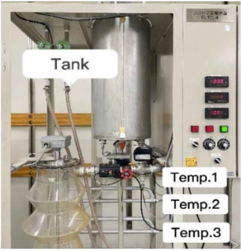
Photo of the temperature control system.
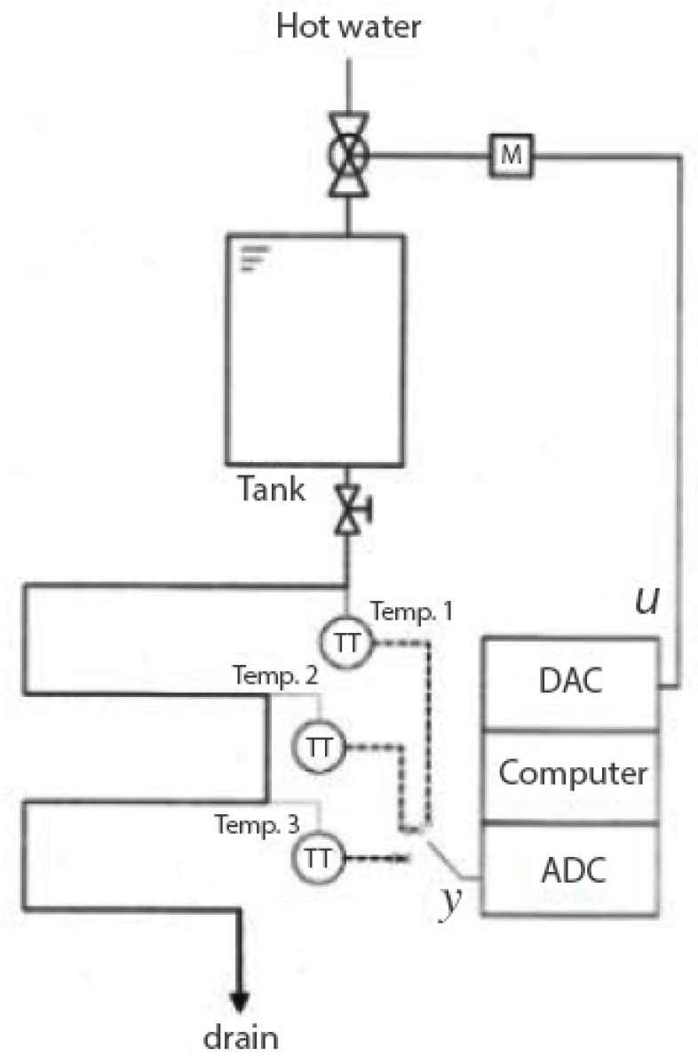
Schematic diagram of the temperature control system.
TS is the sampling time and is set as TS = 5 s in this experiment. Then, the Ziegler-Nichols method [6] is applied considering the stability of the system when the parameters are identified. As a result of the step response, the system parameters are estimated and at the same time the PID parameters can be obtained by applying the Ziegler-Nichols method. The control result by the Ziegler-Nichols method is shown in Figure 9, and the corresponding PID gains are shown as follows:
Control result by the Ziegler-Nichols method.
Firstly, using manually adjusted λ to calculate the PID parameters. When λ = 4.5, the control result is shown in Figure 10. PID gains are shown as follows:
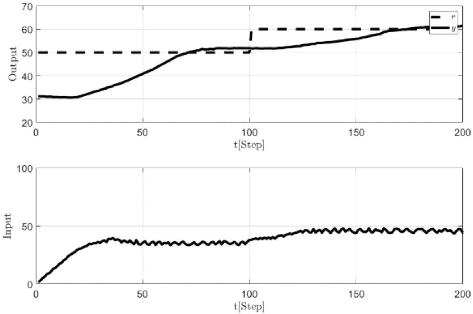
Control result by using manually adjusted λ (λ = 4.5).
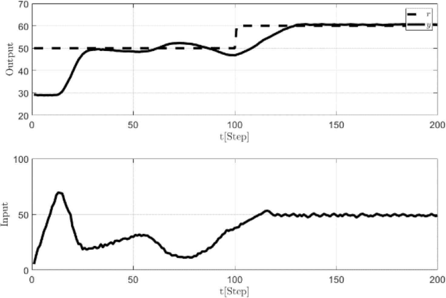
Figure 11 shows the control result when λ = 3.772. In comparing the control results obtained by manually adjusting λ and calculating λ. It is clear that the PID parameters by using the calculated λ can get desirable control performance, and it takes a short time to achieve the control effect. However, the control result by using manually adjusting λ takes a relative long time to reach the target value.
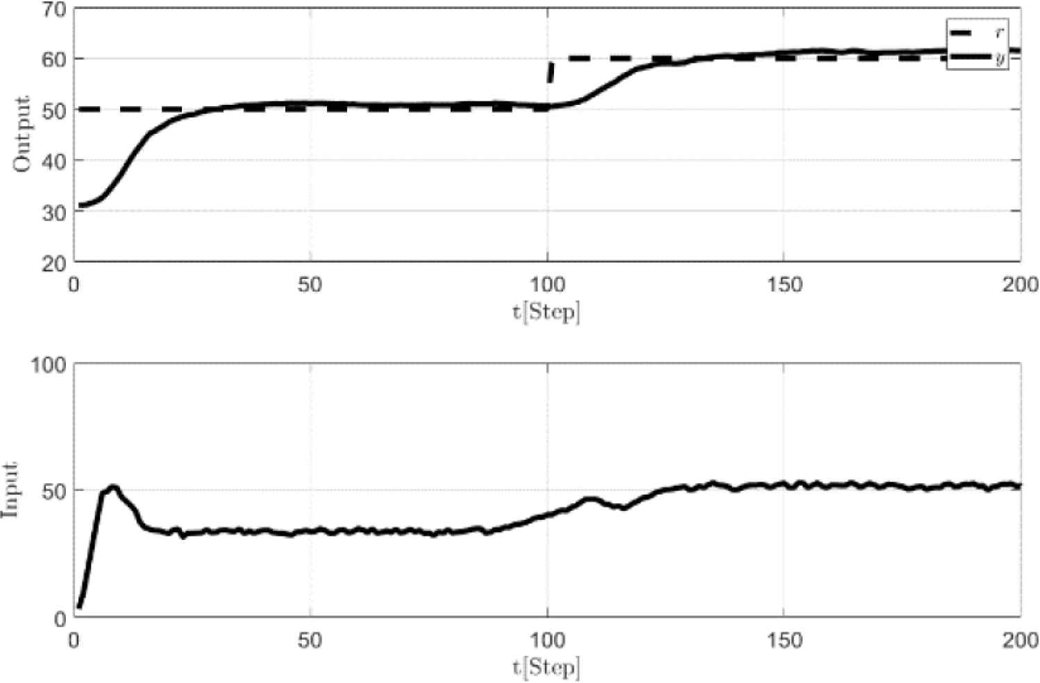
Control result by the proposed method (λ = 3.772).
6. CONCLUSION
In this paper, a design scheme of data-driven GMV-PID controller has been proposed, which can obtain control parameters by applying the Nelder–Mead method based on PID controller. The features of the newly proposed control scheme are summarized as follows:
- •
The user-specified parameter included in GMV-PID control system, is calculated by the NM method for a liner system.
- •
Only using one-short data can calculate λ. The estimation of closed-loop response is introduced in data-driven approach.
- •
The effectiveness of the proposed scheme has been evaluated on the simulation example and experiment.
Furthermore, this system can only calculate linear systems, and future research will be devoted to the development of nonlinear systems.
CONFLICTS OF INTEREST
The authors declare they have no conflicts of interest.
AUTHORS INTRODUCTION
Ms. Liying Shi
 She received her Master’s degree from the Graduate School of Engineering, Hiroshima University, Japan in 2019. Her main research is GMV-PID controller design.
Dr. Zhe Guan
 He received the M.S. degree and D. Eng. degree in Control System Engineering from the Hiroshima University, Japan, in 2015 and 2018, respectively. He is currently working in KOBELCO Construction Machinery Dream-Driven Co-Creation Research Center, Hiroshima University, Japan. He was a visiting postdoc with the Department of Electrical and Computer Engineering, University of Alberta from April to June in 2019. His current research interests are in area of adaptive control, data-driven control, Reinforcement Learning and their applications. He is a member of Society of Instrument and Control Engineers in Japan (SICE).
Prof. Toru Yamamoto
 He received the B. Eng. and M. Eng. degrees from the Tokushima University, Japan, in 1984 and 1987, respectively, and the D. Eng. degree from Osaka University, Japan, in 1994. He is currently a Professor with the Department of Smart Innovation, Graduate School of Advanced Science and Engineering, Hiroshima University, Japan, and a leader of the National Project on Regional Industry Innovation with support from the Cabinet Office, Goverment of Japan. He was a Visiting Researcher with the Department of Mathematical Engineering and Information Physics, University of Tokyo, Japan, in 1991, and an Overseas Research Fellow of the Japan Society for Promotion of Science (JSPS) with the Department of Chemical and Materials Engineering, University of Alberta for 6 months in 2006. His current research interests are in area of self-tuning & learning control, data-driven control, and their implementation for industrial systems. He was a National Organizing Committee Chair of 5th International Conference on Advanced Control of Industrial Processes (ADCONIP 2014) and General Chair of SICE (Society of Instrument and Control Engineers in Japan) Annual Conference 2019, both held in Hiroshima. He is a Fellow of SICE, Institute of Electrical Engineers of Japan (IEEJ) and Japan Society of Mechanical Engineers (JSME).
REFERENCES
Cite this article
TY  - JOUR
AU  - Liying Shi
AU  - Zhe Guan
AU  - Toru Yamamoto
PY  - 2021
DA  - 2021/10/09
TI  - Design of an Optimized GMV Controller Based on Data-Driven Approach
JO  - Journal of Robotics, Networking and Artificial Life
SP  - 180
EP  - 185
VL  - 8
IS  - 3
SN  - 2352-6386
UR  - https://doi.org/10.2991/jrnal.k.210922.006
DO  - 10.2991/jrnal.k.210922.006
ID  - Shi2021
ER  -