
A Design Method of Generalized Predictive Control Systems in Consideration of Noise
- DOI
- 10.2991/jrnal.k.200528.012How to use a DOI?
- Keywords
- Generalized predictive control; closed-loop characteristics; noise; output prediction
- Abstract
Generalized Predictive Control (GPC) is one of the model-based control methods. The control law is derived by minimizing performance index, which includes the squares of control input and the squares of the error between reference signal and output prediction, in order to make the derived control system be stable. Although coprime factorization approach has been used to extend the conventional control law in the previous researches, there has been a possibility that the order of the derived control law becomes high. Therefore, this paper extends GPC through newly-defined output prediction and proposes the method to re-design the control law or the disturbance response with keeping the closed-loop transfer function. Numerical example is shown to check the characteristic of the proposed method.
- Copyright
- © 2020 The Authors. Published by Atlantis Press SARL.
- Open Access
- This is an open access article distributed under the CC BY-NC 4.0 license (http://creativecommons.org/licenses/by-nc/4.0/).
1. INTRODUCTION
Generalized Predictive Control (GPC) [1] is one of the model-based design methods and the closed-loop system is designed through performance index. The performance index includes the error between the reference signal and the output prediction, and the control input. And the closed-loop system is derived by the design parameters for output prediction, future control input series and weighting factor of inputs. For consideration of designing safe systems, although coprime factorization approach [2] has been used in order to extend the control law in the previous researches [3], the derived controller will become high order because a stable polynomial is needed to derive the extended controller. Therefore, this research directly extends generalized predictive control [4] by defining new output prediction and proposes the scheme to re-design the controller without changing the closed-loop characteristics. A numerical example is given to check the characteristics of the proposed method.
2. EXTENSION OF GENERALIZED PREDICTIVE CONTROL
2.1. Conventional GPC
A single-input and -output system is considered for t = 0, 1, 2....
For (1), the following assumptions are hold.
- (i)
km is known.
- (ii)
The pairs of (A[z−1], B[z−1]) and (A[z−1], C[z−1]) are coprime.
- (iii)
C[z−1] is stable polynomial.
The following performance index J is minimized to derive the control law.
In order to derive the control law, the predicted output ŷ(t + j|t) for j = N1 … N2 is calculated by solving the following Diophantine equation.
Multiplying zjΔEj[z−1] to (1) and substituting (6) into it, the following equation is obtained.
2.2. Proposed Method
In conventional GPC, the prediction is defined without including the future noise term Ej[z−1]C[z−1]ξ(t + j). On the other hand, this paper proposes the use of the noise term to date, which can be calculated by (1). Concretely, the following output prediction is newly defined by introducing constant parameter se.
The following equations are considered.
Next, the following equations are defined.
The past and present signals with output and input are also defined by
From these equations, the output prediction can be expressed as the following equation, which separates the input term Rj[z−1]Δu(t + j − km) in the current and future time from the other signal
The following vectors and coefficients at time t are defined for j = N1,…, N2.
Then the output prediction (15) can be expressed as following vector form.
By using the above equation, the performance index J can be described as follows.
Minimizing the performance index J for the input vector U, the control input can be given.
The following vector and polynomials are defined.
Then the transfer function of control law is expressed as follows.
Moreover, the following polynomials are defined.
Then the closed-loop system can be derived as follows.
It means that the output response is the same as the conventional GPC. On the other hand, it can find that the disturbance response can be tuned through the design polynomial
3. NUMERICAL EXAMPLE
The following controlled plant is considered as Okazaki et al. [5].
The number of simulation steps is 500, the initial values of input and output are set to be 0, and the variance of ξ(t) is σ2 = 0.001 (each data of noise ξ(t) is the same for the conventional and the proposed method). The reference signal w(t) is 0.1. The design parameters of GPC are given as follows.
In this example, the design parameter of the proposed method is given as se = −1.8.
Figures 1 and 2 show the conventional output and input. In Figure 1, the dashed line and solid line mean the reference signal w(t) and the output signal y(t) respectively. In Figure 2, the upper figure shows the control input u(t) and the lower one shows the input increment Δu(t). Figures 3 and 4 show the proposed output and input. Their lines are the same meanings as conventional method. From these figures, it can find that the proposed method can change the noise influence on output.
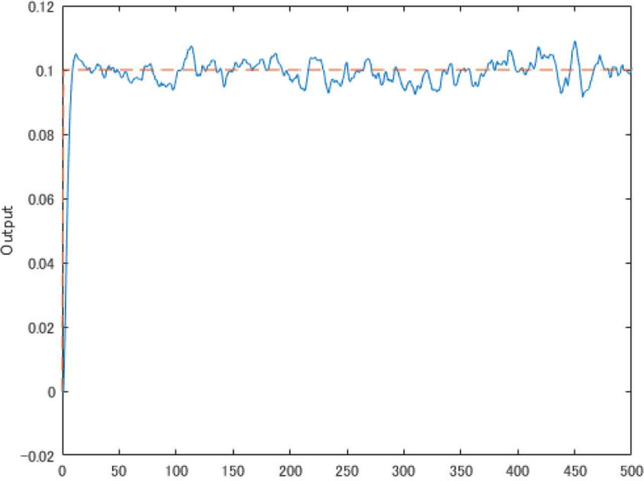
Conventional output.
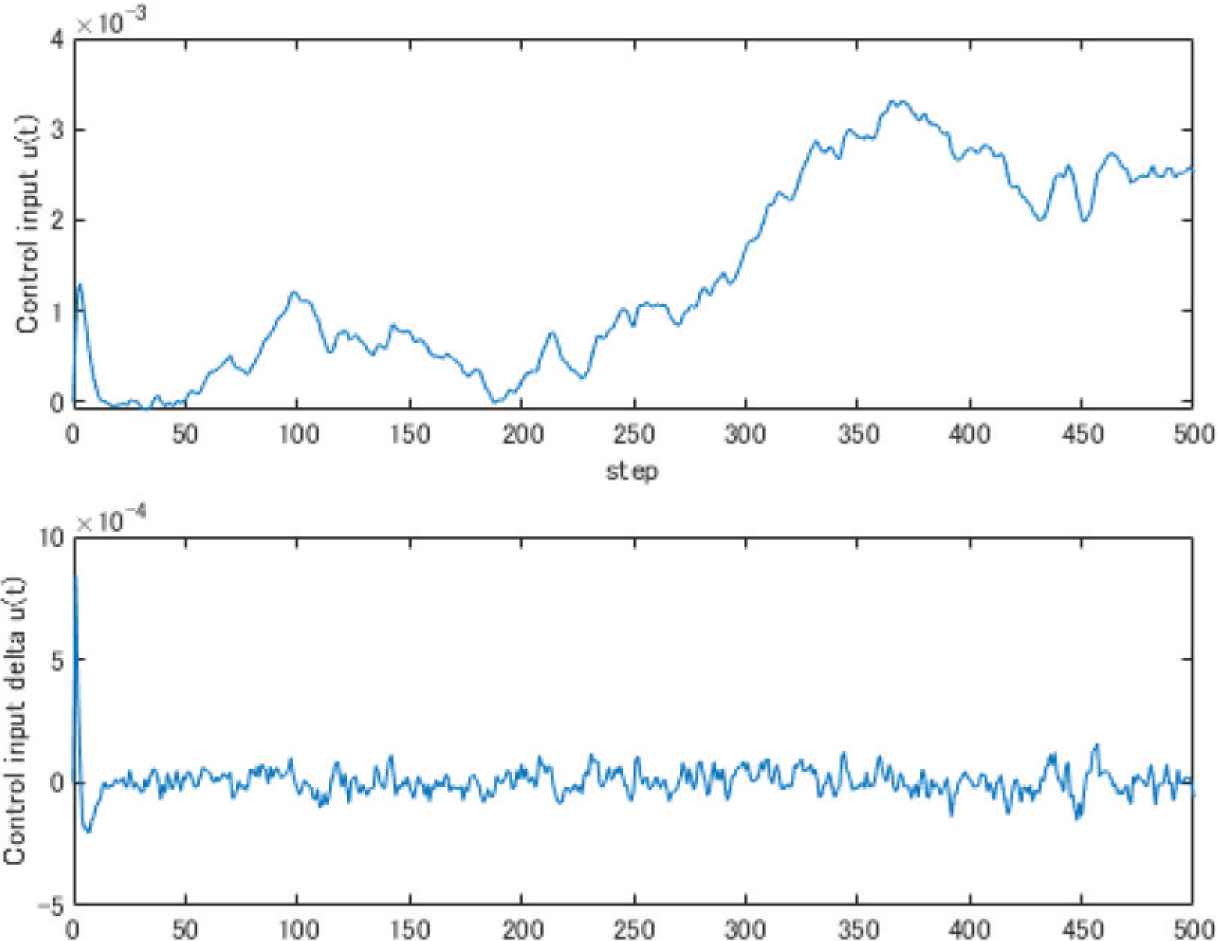
Conventional input.
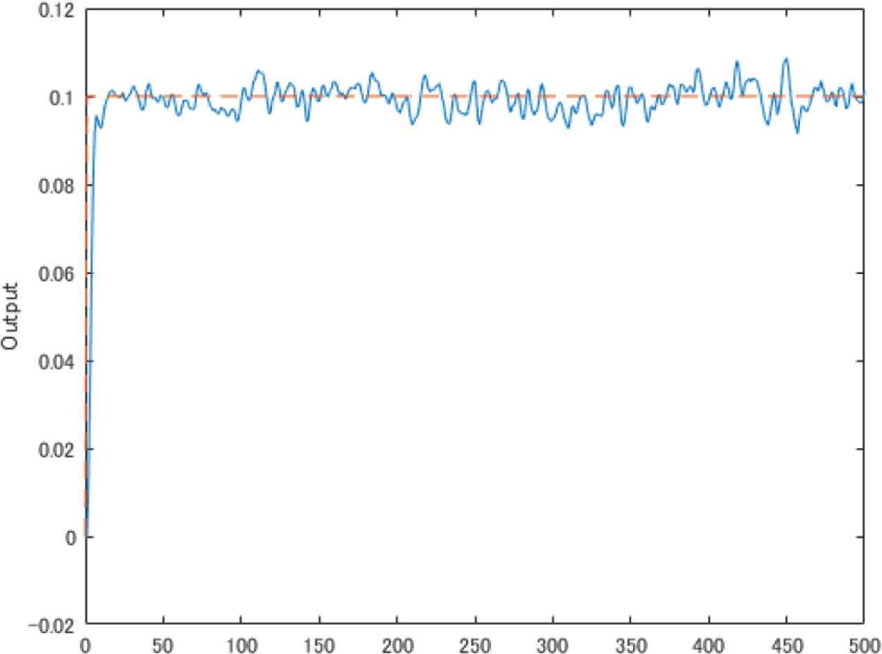
Proposed output.
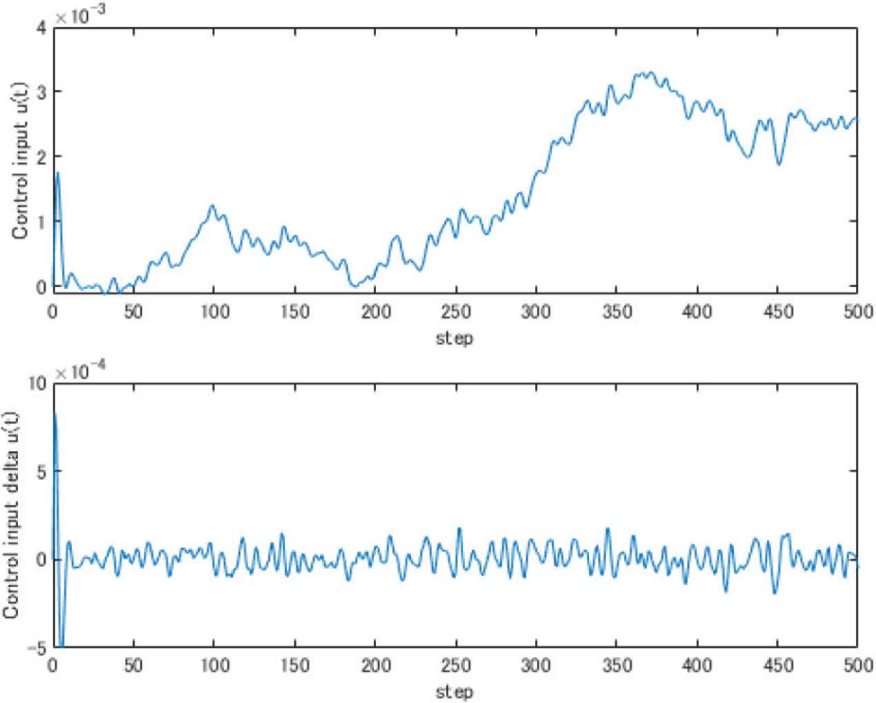
Proposed input.
4. CONCLUSION
This paper proposed a directly extended method of conventional GPC through newly-defined output prediction. The derived control law can re-design the characteristic from noise to output with keeping the closed-loop transfer function. Numerical example was given to check the characteristic of the proposed method.
As future work, the selection method of design parameter se should be considered.
CONFLICTS OF INTEREST
The author declares no conflicts of interest.
AUTHOR INTRODUCTION
Dr. Akira Yanou
 He received his PhD in Engineering from Okayama University, Japan in 2001. He worked with School of Engineering, Kinki University from 2002 to 2008, and Graduate School of Natural Science and Technology, Okayama University from 2009 to 2016. He joined Department of Radiological Technology, Kawasaki College of Allied Health Professions in 2016, and Faculty of Health Science and Technology, Kawasaki University of Medical Welfare in 2017, as an Associate Professor. His research interests include adaptive control, strong stability systems and estimation.
REFERENCES
Cite this article
TY  - JOUR
AU  - Akira Yanou
PY  - 2020
DA  - 2020/06/03
TI  - A Design Method of Generalized Predictive Control Systems in Consideration of Noise
JO  - Journal of Robotics, Networking and Artificial Life
SP  - 129
EP  - 132
VL  - 7
IS  - 2
SN  - 2352-6386
UR  - https://doi.org/10.2991/jrnal.k.200528.012
DO  - 10.2991/jrnal.k.200528.012
ID  - Yanou2020
ER  -