
Pulse Point Position Tracking-control and Simulation based on 4-DOF Pulse Diagnosis Robot
- DOI
- 10.2991/jrnal.k.190828.009How to use a DOI?
- Keywords
- Pulse diagnosis; robot; follow control; simulation
- Abstract
Pulse diagnosis has been proved to be of great practical value in the past dynasties. The key of high-quality pulse diagnosis is how to dynamically adjust the vertical relationship between the pulse and the sensor dynamically. The design adopts a four degree of freedom manipulator combined with a matrix sensor to form a diagnostic robot, so as to achieve rapid adjustment and keep the diagnostic pulse sensor perpendicular to the pulse. As a result, kinematics analysis and simulations can be performed and the feasibility of the results can be showed as well.
- Copyright
- © 2019 The Authors. Published by Atlantis Press SARL.
- Open Access
- This is an open access article distributed under the CC BY-NC 4.0 license (http://creativecommons.org/licenses/by-nc/4.0/).
1. INTRODUCTION
For more than 2000 years, pulse diagnosis has played a very important role in the practice of diagnosis and treatment [1]. The theory of pulse diagnosis has been applied through the physiology, pathology, diagnosis, treatment and other aspects of Chinese medicine. The quality of pulse diagnosis is related to the effect of “syndrome differentiation and treatment” in all clinical departments, which is of great significance to the guidance of Traditional Chinese Medicine (TCM) theory in medical practice. Since the 1960s, with the development of modern science and technology, many domestic and foreign researchers have been committed to promoting the modernization of TCM pulse diagnosis and expected to improve the situation of “difficult to identify” by using modern medical instruments [2].
2. COMPOSITION OF THE PULSE DIAGNOSIS ROBOT
The key of high-quality pulse diagnosis is how to dynamically adjust the vertical relationship between the pulse and the sensor (only the vertical relation between sensor and pulse can guarantee the accuracy of pulse diagnosis). The robot is made up of a Four Degree of Freedom (4-DOF) manipulator and a pulse diagnosis sensor matrix, as shown in Figures 1 and 2.
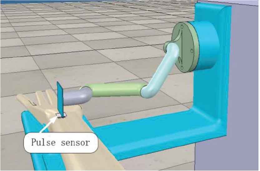
The robot which is made up of a 4-DOF manipulator and a pulse diagnosis sensor matrix.
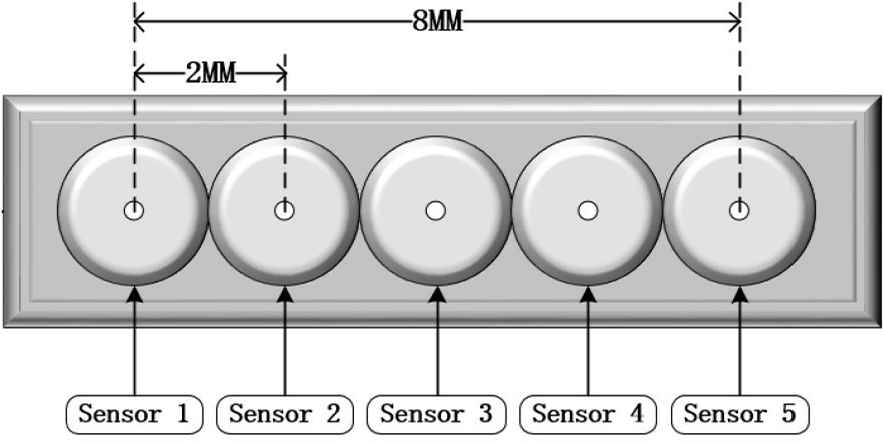
The pulse diagnosis matrix sensor is composed of five pressure sensors in a row. The matrix sensors are fitted on the end of the manipulators.
3. KINEMATICS OF THE 4-DOF MANIPULATOR
According to the standard D–H parameter table method, the coordinate system of the manipulators is shown in Figure 3. The coordinate system 1 is coinciding with the origin of the base coordinate system 0, and the origin of the coordinate system of the pulse sensor coincides with the origin of the wrist coordinate system. The D–H parameters are obtained as shown in Table 1.
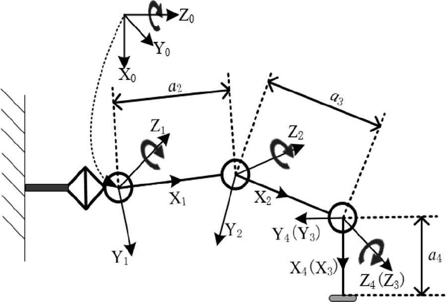
Manipulators structure and its coordinate systems of joints.
| i | αi | ai | di | θi |
|---|---|---|---|---|
| 1 | −π/2 | 0 | 0 | θ1 |
| 2 | 0 | a2 | 0 | θ2 |
| 3 | 0 | a3 | 0 | θ3 |
| 4 | 0 | 0 | 0 | θ4 |
Parameters of D–H
The length of the connecting rod is ai: the distance from the Zi−1 axis to the Zi axis is moved along the Xi axis. The angle of the connecting rod is αi: the angle of rotation of the Zi−1 axis to the Zi axis around the Xi axis. Connecting rod offset di: along the Zi−1 axis, the distance between the Xi−1 axis and the Xi axis is moved. Joint angle θi: around the Zi−1 axis, rotate the Xi−1 axis to the angle of the Xi axis.
3.1. Forward Kinematics of the Manipulator
According to the standard D–H parameter method, the general equation of the link homogeneous transformation matrix is [Equation (1)]:
From Equation (1) and the established D–H parameter table, the homogeneous transformation matrix equation of each adjacent joint can be obtained [Equation (2)]:
3.2. Inverse Kinematics of the Manipulator
The common methods of inverse kinematics solving mainly include algebraic method and geometric method [3]. Compared with the algebraic method, the geometric method has advantages of simple calculation and avoids the discussion of range of values by using the constraint relationship between the joints [4]. In this paper, the inverse kinematics of the 4-DOF pulse diagnosis robot is solved by geometric method [5].
Before solving the kinematics with the geometric method, the first rule is that θ1 has rotated to a position parallel to the target position. According to the establishment rule of D–H, the schematic diagram of the plane based on the geometric method can be obtained as shown in Figure 4.
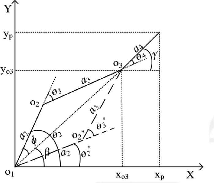
Geometric relationship of three joints in XY-plane.
Assuming that the position coordinates (xp, yp) of the end point P and the azimuth angle γ of the point P are known. According to the geometric relation, Equations (3) and (4) can be drawn that:
By using the cosine theorem in Δo1o2o3, Equations (5), (6) and (7) can be drawn that:
4. MODELING AND SIMULATION
4.1. Modeling in V-REP
The robot model is established in Virtual Robot Experimentation Platform (V-REP) as shown in Figure 1. Setting the parameters of the robot model: a2 = 0.08 m, a3 = 0.1 m, a1 = −90°. The initial posture of the robot can be calculated by assigning the angle of each joint to 0° as shown in Equation (8):
This data we got is identical to the data obtained in the V-REP simulation.
The pulse diagnosis matrix sensor adopted in this simulation is composed of five pressure sensors in a row, which is shown in Figure 5a. Each point of the sensors can sense the corresponding pulse. In the simulation, the pulse sensor is exposed to the pulse at different positions to obtain the simulation data. By analyzing the data, the relative pose of sensors with respect to the pulse can be drawn, which will be used to adjust the posture of the joints.
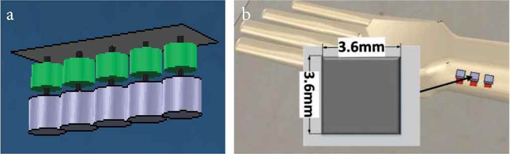
Pulse sensor and pulse model in V-REP. (a) Pulse sensor model. (b) Pulse model.
Pulse model is also established with similar dynamic properties to the human pulse, as shown in Figure 5b. The width of the pulse model is set as 3.6 × 3.6 mm2 according to average adult’s size.
4.2. Pulse Detect Simulation
In the V-REP simulation, the pulse beat curve at different positions is measured with changing the relative position of the pulse matrix sensor relative to the pulse model. When the first sensor of the pulse matrix sensor is aligned with the pulse model, the pulse curve obtained is shown in Figure 6. It is quite obvious from the figure that the value of sensor 1 is the largest, and the center of the pulse matrix sensor is not perpendicular to the pulse model.
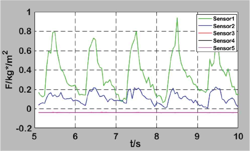
The first sensor is aligned with the pulse.
When the third sensor of the pulse matrix sensor is aligned with the pulse model, the pulse curve is shown in Figure 7. It is clear that the intensity of sensors 2–4 are same to each other. When the curve similar to Figure 8 is obtained, the pulse matrix sensor can be considered as perpendicular to the pulse, and the third sensor is aligned with the pulse.
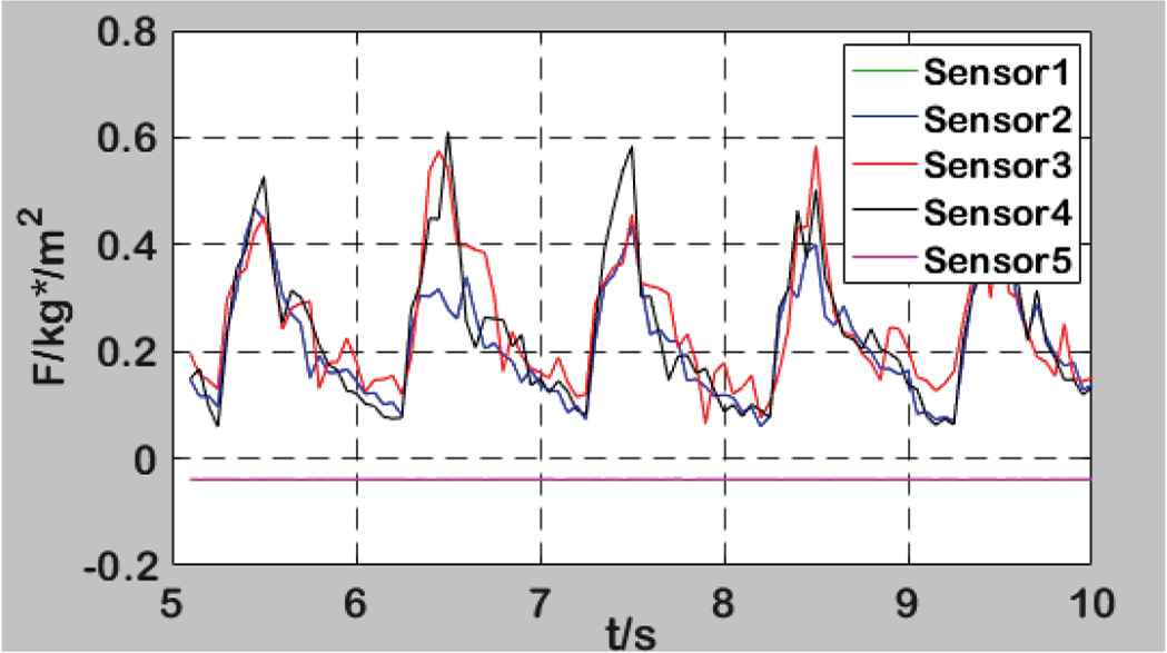
Beating curves of sensors when the third sensor is aligned with the pulse.
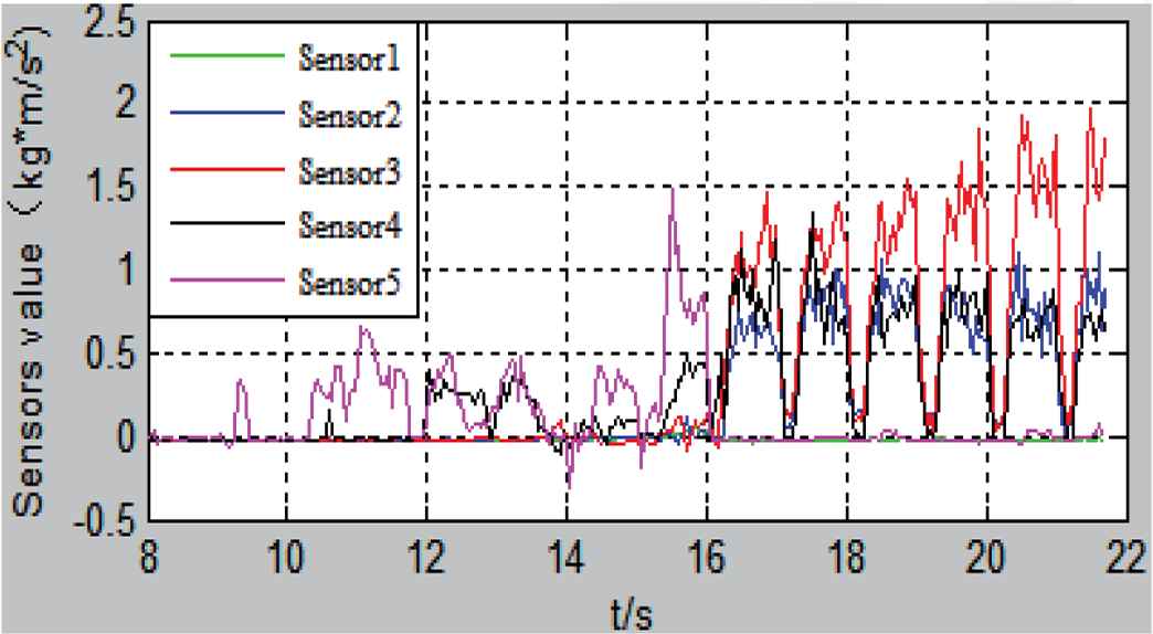
Curve change of each sensor point during pulse pose tracking control.
4.3. Pulse pose tracking control simulation
Figure 8 shows that the posture curves of the pulse sensors. The values changes related to the relative position between sensors and the pulse, until the matrix sensor is perpendicular to the pulse, and sensor 3 is aligned with the pulse. Figure 9 shows that the joints were adjusted to move from sensor 5 to sensor 3, and finally sensor 3 is perpendicular to the pulse as expected.
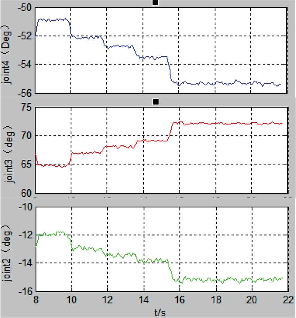
Curve change of θ2, θ3, and θ4 during pulse pose following control.
5. CONCLUSION
In this paper, a diagnostic robot with a 4-DOF manipulator and a pulse diagnosis matrix sensor was introduced. The kinematic was analyzed and the model was simulated on V-REP. The simulation results show that the proposed robot can find the position of pulse and adjust the joints to the posture as expected according to the feedback information from the pulse diagnosis matrix sensor.
CONFLICTS OF INTEREST
The authors declare they have no conflicts of interest.
ACKNOWLEDGMENT
This work is partially supported by
Authors Introduction
Dr. Qunpo Liu
 He graduated from the Muroran Institute of Technology (Japan) with a PhD in Production Information Systems. He is an Associate Professor at the School of Electrical Engineering at Henan Polytechnic University (China) and a master’s tutor. He is mainly engaged in teaching and research work in special environment mobile robots, intelligent instruments and industrial automation equipment.
Mr. Guanghui Liu
 He graduated from Henan Polytechnic University (China) in 2018 with a bachelor’s degree in automation. He is currently studying for a master’s degree in Control Engineering at Henan Polytechnic University. He is mainly engaged in research on pulse diagnosis robot.
Dr. Hongqi Wang
 He is an Associate Professor at the School of Electrical Engineering, Henan Polytechnic University (China), as well as a tutor for postgraduate students. His main research direction is robot control.
Mr. Xianzhe Liu
 He is currently studying for a bachelor’s degree in automation at Henan Polytechnic University (China). He is mainly engaged in modeling and simulation of robot.
Dr. Naohiko Hanajima
 He graduated from the Hokkaido University (Japan) of Technology in Japan with a PhD. He is a Professor at the College of Information and Systems at Muroran Institute of Technology (Japan). He is mainly engaged in robotics and intelligent equipment.
REFERENCES
Cite this article
TY  - JOUR
AU  - Qunpo Liu
AU  - Guanghui Liu
AU  - Hongqi Wang
AU  - Xianzhe Liu
AU  - Naohiko Hanajima
PY  - 2019
DA  - 2019/09/11
TI  - Pulse Point Position Tracking-control and Simulation based on 4-DOF Pulse Diagnosis Robot
JO  - Journal of Robotics, Networking and Artificial Life
SP  - 113
EP  - 117
VL  - 6
IS  - 2
SN  - 2352-6386
UR  - https://doi.org/10.2991/jrnal.k.190828.009
DO  - 10.2991/jrnal.k.190828.009
ID  - Liu2019
ER  -