
Game Theoretic Strategies for Supplier Capability Assessment and Manufacturing Order Allocation
 , Yu-Min Chuang2
- DOI
- 10.2991/jracr.k.201014.002How to use a DOI?
- Keywords
- Supplier power value; Nash equilibrium; Shapley value; supplier allocation
- Abstract
An effective method is required to determine the amount and priority for the deployment of suppliers for multiple manufacturing processes, particularly when the available budget for each manufacturing process is limited. In this study, we propose an integrated approach for supplier assessment that consists of two game theory models which are designed to recommend manufacturers on how best to choose suppliers given budgetary limitations. In the first model, the interactive behaviors between the key factors representing the manufacturer and the supplier are modeled and analyzed as a two-player and zero-sum game, after which the Supplier Power Value (SPV) is derived from the pure or mixed strategy Nash equilibrium. In the second model, 12 SPVs are used to compute a Shapley value for each supplier, in terms of the thresholds of the majority levels in one manufacturing process. The Shapley values are then applied to create an allocated set of limited manufacturing orders for suppliers. The experimental results present that the manufacturer can use our approach to quantitatively evaluate the suppliers and easily allocate suppliers within one manufacturing process.
- Copyright
- © 2020 The Authors. Published by Atlantis Press B.V.
- Open Access
- This is an open access article distributed under the CC BY-NC 4.0 license (http://creativecommons.org/licenses/by-nc/4.0/).
1. INTRODUCTION
With the globalization of supply chain management, organizations have to find ways to reduce costs through global sourcing, to increase their competitive advantage. Supplier evaluation or selection plays an important role in the manufacturing process, particularly when the available budget is restricted in manufacturer expenditures. Each enterprise might have its supplier selection criteria, and from these criteria devise their method of selection [1]. Each supply chain includes a number of manufacturers, with finite budgets, which need to be allocated to all suppliers in all parts of the manufacturing process. Some manufacturers are faced with budgetary limitations. Each manufacturer has multiple suppliers each of which in turn possesses different specific capabilities (such as delivery performance and cost of manufacturing). Supply Chain Management (SCM) is thus needed to perform a feasible allocation of suppliers during manufacturing process flows.
Poirier and Reiter [2] explained that each member of the supply chain channel which extends from the supplier to the customers must be integrated into the design for marketing, procurement, distribution, and other activities of each organization. Dickson [3] used questionnaire responses to identify 23 factors of influence for supplier selection criteria. Their study showed product quality, delivery, and past performance history to be critical factors in supplier selection. Weber et al. [4] found in a study of vendor selection that suppliers of equipment, output capacity, and technological capability are also related to supplier evaluation for the manufacturing process. Chan et al. [5] and Maurizio et al. [6] indicated that the cost of the product, which measures supplier capability from the perspective of the supplier, is crucial to support the manufacturing flow.
There is a trade-off between increased manufacturer performance and a decrease in manufacturing costs in the selection of multiple suppliers in SCM. Manufacturer performance shows an upward slope in Figure 1 but manufacturer demand states that all other factors remaining equal, supplier service quality is better with higher manufacturer demand, because higher service quality improves manufacturer performance. In other words, the lower the manufacturer’s demand, and the worse the service quality, leading to reduce manufacturer performance. The downward slope in Figure 1 indicates that the lower the manufacturer demand, the lower the cost that will be spent on that good. In other words, a smaller manufacturer demand produces higher supplier service quality which results in decreasing cost to the manufacturer; see the downward slope. Jayaraman et al. [7] indicated that it is more likely to produce high-quality, low-cost products with the capabilities of suppliers and the requirements of manufacturers. This means that the ideal of high-level manufacturer performance and low-level budgets is difficult to achieve. Consequently, we need to find the balance between lower cost (or budgets) and higher manufacturer performance; see Figure 1.
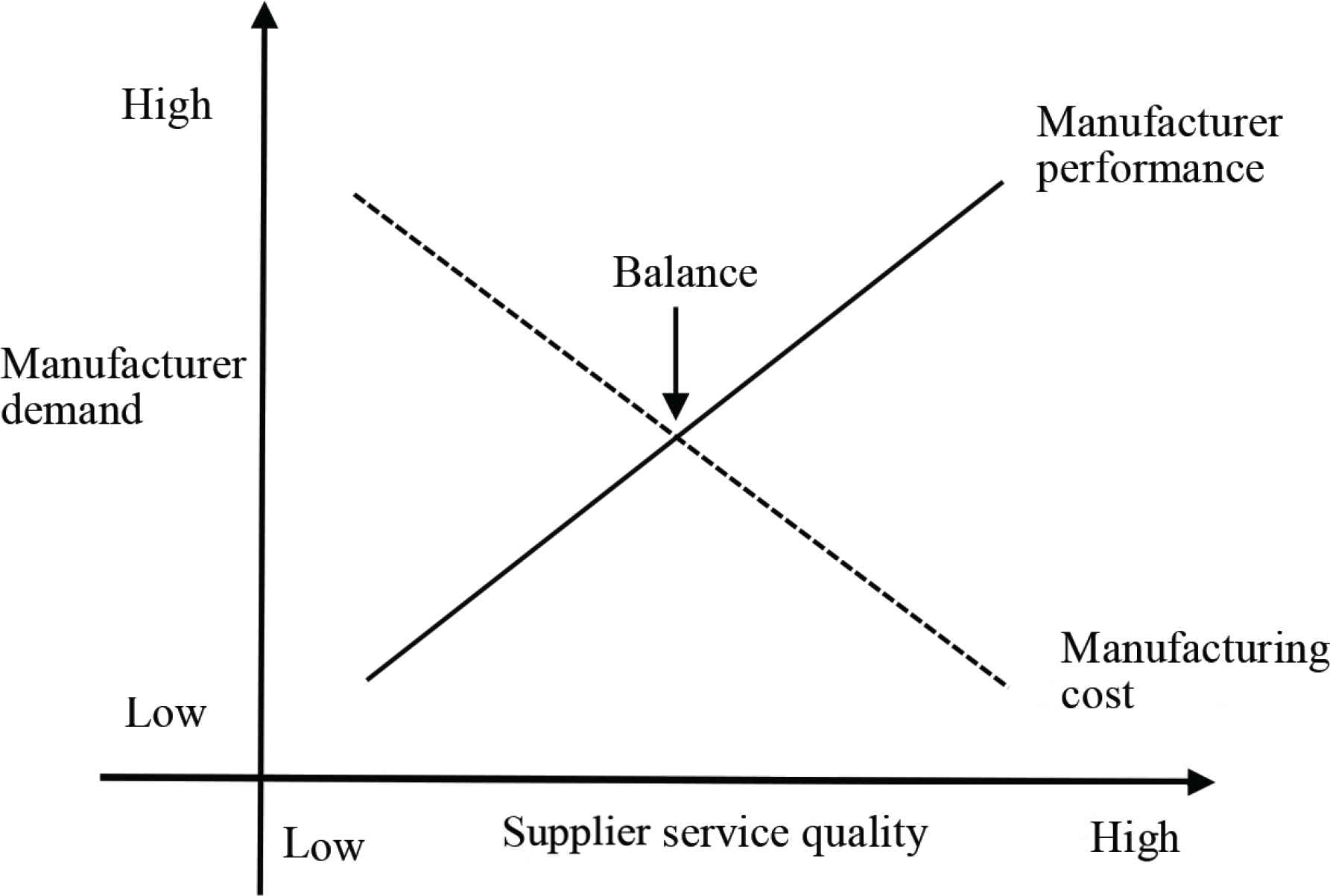
The balance between lower budgets and higher manufacturer performance in SCM.
In previous research, the supplier selection process has been investigated taking the manufacturer’s interests as the starting point but ignoring the point of views from the suppliers. This study applies a two-stage game model to solve the supplier allocation problem. First, we establish the interactions between the manufacturer and the supplier as a two-player strategy, in a non-cooperative finite and zero-sum game. The proposed payoff functions are calculated by the competency measures (i.e., manufacturer’s requirements and supplier’s capabilities) for four assessment of factors (i.e., quality of products, cost of manufacturing, the technology of the supplier, and delivery performance) affecting the manufacturing flow. The Supplier Power Value (SPV) is derived from the payoff matrix. In the second model, a manufacturing process of all suppliers is playing a cooperative game. The Shapley value is adopted as a measure to calculate the marginal contribution of all suppliers in the manufacturing process and the mutually agreed upon the allocation of manufacturing budgets. Multiple suppliers are united into the coalition groups for calculation of the majority thresholds in such a way as to distribute fair and feasible supplier deployment in a single manufacturing flow. In the experimental simulation, the proposed models are applied to compute the SPV for each supplier and verify that the Shapley value does indeed offer significant assistance for the purpose of decision-making and efficient allocation of suppliers in the supply chain.
2. LITERATURE REVIEW
Within the past few decades, researchers have developed a variety of optimization methods in order to optimize multi-supplier selection and order quantity allocation, to improve supply chain performance. Hosseini and Barker [8] considered three resilience-based supplier selection criteria: absorptive (e.g., surplus inventory), adaptive (e.g., rerouting), and restorative (e.g., technical resource restoration) capacities in their development of a Bayesian network formulation for supplier evaluation and selection. Their model depended upon expert judgment. In addition, Bayesian networks are usually very complicated because of the large number of variables used to capture causality.
Dogan and Aydin [9] proposed an integrated model which provides some advantages when analysing supplier selection problems. Their goal was to identify uncertainties more clearly and utilizes the buyer’s specific domain knowledge. They provided a supplier assessment and selection process for first-tier suppliers in the automotive industry, but their model also relies upon expert opinions and judgments.
Erdem and Göçen [10] developed an analytic hierarchy approach, which captured both qualitative and quantitative criteria for supplier evaluation, including cost, quality, logistics, and technology. Based on these factors of assessments, a goal programming model was proposed to distribute orders among suppliers. Their model has been applied to the decision support system, which presents dynamic, flexible, and fast decision-making.
Mohammed et al. [11] and Nazari-Shirkouhi et al. [12] proposed a fuzzy analytic hierarchy process. The multi-objective programming model adopt the final Pareto solution to choose suppliers in a supply chain under various uncertainties (such as cost, demand).
Scott et al. [13] proposed a three-stage decision support system. Their first stage process is run for supplier evaluation and selection according to the stakeholders’ requirements, evaluation criteria, and supplier’s characteristics (i.e., capacity, price, quality criteria), after which the supplier performance score is derived for each supplier. In the second stage, the optimization algorithm is used for order allocation based on the supplier performance score. In the third stage, their decision support system is validated using a Monte-Carlo simulation.
Mendoza and Ventura [14] proposed the nonlinear programming model that selects the best supplier set and determines the appropriate order quantity allocation, given the supplier’s ability and quality constraints so as to minimize annual ordering, inventory holdings, and procurement costs. Demirtas and Üstün [15] also proposed a two-stage model that utilizes tangible and intangible elements when selecting the best supplier and defines the best quantity among the selected suppliers to maximize the total value of the purchase and minimize defect rate. Four different plastic molding companies working with refrigerator factories were analysed according to 14 criteria grouped into four clusters: benefits, opportunities, costs, and risks.
Huang et al. [16] proposed a solution concept derived from cooperative game theory (i.e., Shapley value) to obtain the marginal contributions of suppliers so as to select the best suppliers. Wang and Li [17] expanded supplier evaluation in the case of variable returns to scale for the development of a new Nash bargaining game, including a Data Envelopment Analysis (DEA) model for supplier evaluation. Their model uses universal weights for evaluation based on the Nash bargaining game DEA model can fairly evaluate and rank all suppliers. All suppliers are motivated to accept Pareto solutions for Nash bargaining games.
The above supplier evaluation and order allocation methods are designed for improving the supply chain performance with more complicated calculations. This study extends the supplier evaluation model of Wu et al. [18] to more explicit in which the interactions between manufacturer and supplier are combined with manufacturing requirements. The interactions of six critical factors (i.e., quality of products, cost of manufacturing, the technology of the supplier, delivery performance, service demand, and priority) between the supplier and the manufacture are modelled and analysed as a non-cooperative game to create a SPV with which to evaluate a given supplier. And then the Shapley value is applied in a simple cooperative game to easily and quickly calculate a fair manufacturing order allocation based on the SPV.
When the supply chains face unpredictable damage caused by sudden natural disasters (such as the outbreak of COVID-19, hurricanes or earthquakes), or man-made threats (such as terrorist attacks or strikes), they need to meet customer requirements and recover from the interruption [19,20]. Hosseini et al. [21] proposed a supply chain resilience method that integrated Markov chain and dynamic Bayesian network methods to find the potential high-risk paths in the supply chain and to prioritize the emergency response and recovery strategies. One contribution of the proposed approach as compared to these above researches is that we consider the interactions between the manufacturer and the supplier in a supplier assessment game, which fairly and reasonably distributes manufacturing budgets.
3. THE PROPOSED FRAMEWORK
The two models proposed here consider a 12-supplier, one manufacturing process of the manufacturer; see Figure 2. Two games are constructed for the economical allocation of suppliers. One is a supplier assessment game which calculates 12 SPVs during one manufacturing process. The other is a manufacturing order allocation game which efficiently distributes the limited manufacturing orders to all suppliers within one manufacturing process. A simplified workflow chart outlining the principles of the supplier deployment model for this manufacturing process appears in Figure 2. In the first step, the interactions between the manufacturer and the supplier are modelled as a two-player, zero-sum, and non-cooperative game. After considering the information needed to evaluate each supplier, such as the quality of the products, cost of manufacturing, the technology of the supplier, delivery performance, and the manufacturer’s requirements (i.e., services demanded and priority), the first model calculates two player’s payoff for their strategy combination in the matrix. Given the payoff matrix, a unique SPV is calculated for each supplier from the expected payoff using the pure (or mixed strategy) Nash equilibrium. In the second step, a cooperative game model (i.e., manufacturing order allocation game) is applied to generate a power index for the deployment of suppliers based on the Shapley value. From the total SPVs of all suppliers, the majority of SPV values is computed to generate the majority threshold in one manufacturing process. Then the 12 Shapley values (s1, s2, …, s12) are calculated based on the threshold. Finally, the proposed model generates the appropriate manufacturing order allocation vector (e1, e2, …, e12) for the allocation of the suppliers to a manufacturer in the supply chain.
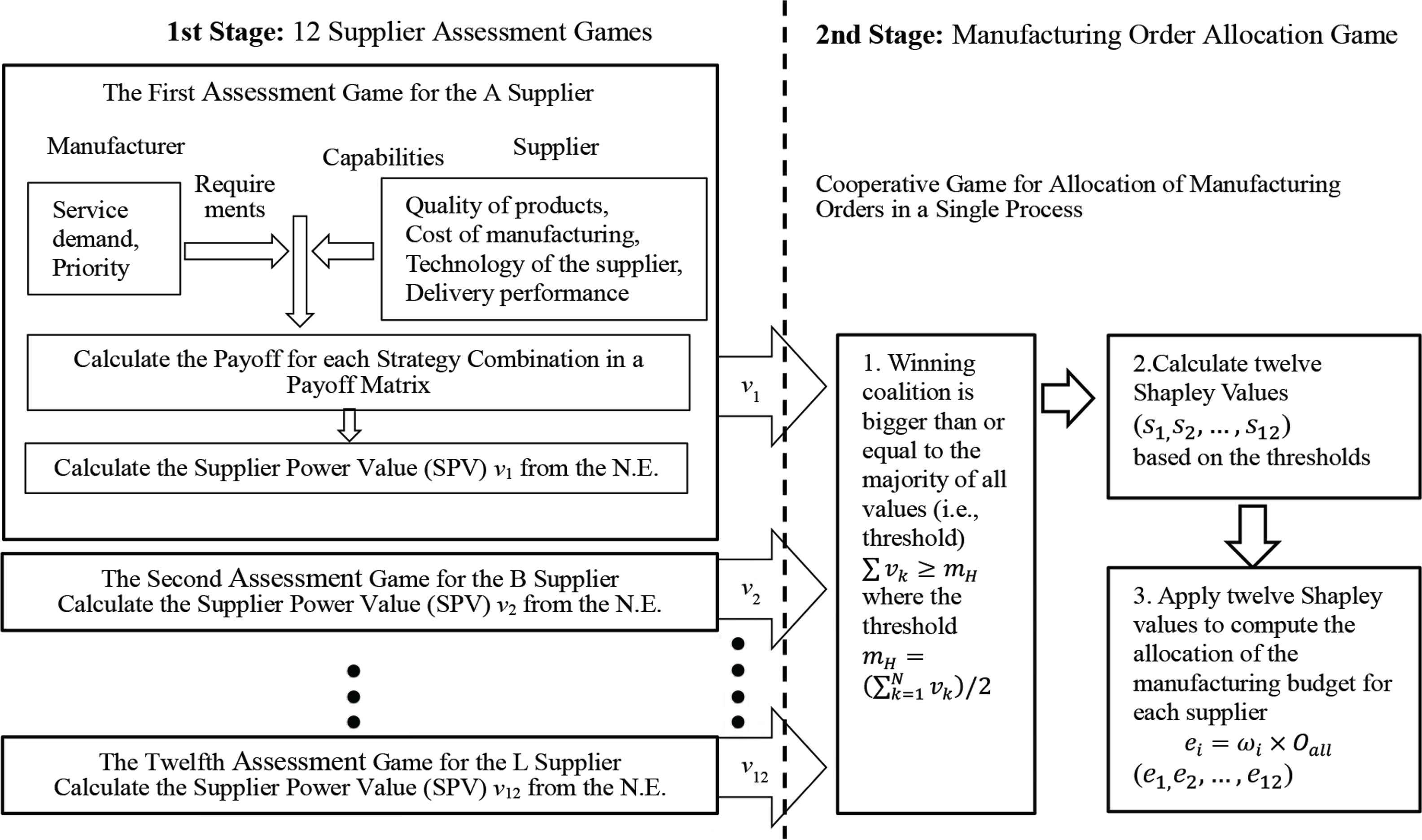
Workflow for supplier capability assessment and manufacturing order allocation.
3.1. Twelve Supplier Assessment Games
From the 12 supplier assessment games in the first stage, we obtain SPVs for the suppliers, i = 1, 2, …, 12. In each simultaneous game, two players implement a single static step. Manufacturer and supplier behaviours are captured with a two-person and zero-sum game. It is assumed that the manufacturer and the supplier are rational players. They form a set of noncooperative players I = {I1, I2}, where I1 is the manufacturer evaluating supplier capability; and I2 is the supplier. Dickson [3] conducted a questionnaire survey of about 300 commercial organizations (mainly manufacturing companies), asking the purchasing managers of these companies the question: What are the important factors in choosing a supplier. He found that quality, price, delivery, technical capabilities, and service are the most critical factors in the supplier selection. Cheraghi et al. [22] also reviewed more than 110 research papers to find these five critical factors for successful supplier selection. The parameters for determining the measures for evaluating a good supplier are defined below.
Assume that the manufacturer is player 1 in a supplier assessment game. Each manufacturer has a decision maker, who in turn has specific suppliers with which to prepare for product manufacturing processes. Here, U denotes the set of player 1’s strategies: U = {u1, u2} = {services demand, priority}. The greater the productivity of the manufacturing process, the larger the supplier capacities needed. W denotes the set of manufacturer service requirements for each manufacturing process in a supply chain. W = {w1, w2, w3, w4}. The variable wk denotes the number of product manufacturing services required u1 with the suppliers’ capacity dk, k = 1 – 4, where wk = 1 is the lowest level and wk = 4 is the highest, as shown in Table 1. Each supplier is assigned a priority P on a scale of 1–4 indicating the significance of the supplier’s capacity dk. P denotes the set of manufacturer priority requirements for each manufacturing process in a supply chain, P = {p1, p2, p3, p4}. The variable pk denotes the manufacturing priority required u2 with the suppliers’ capacity dk, k = 1–4, where pk = 1 is the lowest level and pk = 4 is the highest, as shown in Table 1. Player 1 has two strategies and player 2 has four strategies in this game, therefore there exists 36 (4! × 4!) potential combinations. This study presents six cases in the simulation; see Table 1.
| No | Manufacturer (player 1) | Supplier (player 2) | |||
|---|---|---|---|---|---|
| Quality of products | Cost of manufacturing | Delivery performance | The technology of the supplier | ||
| Case 1 | Service demand | 1 | 3 | 2 | 4 |
| Priority | 4 | 1 | 3 | 2 | |
| Case 2 | Service demand | 4 | 1 | 2 | 3 |
| Priority | 1 | 2 | 3 | 4 | |
| Case 3 | Service demand | 3 | 2 | 4 | 1 |
| Priority | 1 | 4 | 2 | 3 | |
| Case 4 | Service demand | 1 | 4 | 3 | 2 |
| Priority | 4 | 2 | 1 | 3 | |
| Case 5 | Service demand | 3 | 4 | 2 | 1 |
| Priority | 1 | 2 | 4 | 3 | |
| Case 6 | Service demand | 1 | 3 | 4 | 2 |
| Priority | 4 | 1 | 2 | 3 | |
Manufacturer X’s requests for service demand and priority: six cases
The supplier is player 2 and D denotes the set of player 2’s strategies: D = {d1, d2, d3, d4} = {quality of products, cost of manufacturing, the technology of the supplier, and delivery performance}. C denotes the set of capacities available from one supplier: C = {c1, c2, c3, c4}. ck denotes the number of capacities available at the supplier’s capacity dk, k = 1–4, where ck = 1 is the lowest level and ck = 10 is the highest, as shown in Table 2.
| Level | Quality of products (c1) (%) | Cost of manufacturing (c2) | Delivery performance (c3) (%) | The technology of the supplier (c4) [23] |
|---|---|---|---|---|
| 10 | 100 | (Manufacturer’s accepted price)/(Supplier’s offer Price) * 10 | 100 | 2 ≦ c4 |
| 9 | 98 | 98 | 1.83 ≦ c4 < 2 | |
| 8 | 96 | 96 | 1.67 ≦ c4 < 1.83 | |
| 7 | 94 | 94 | 1.5 ≦ c4 < 1.67 | |
| 6 | 92 | 92 | 1.33 ≦ c4 < 1.5 | |
| 5 | 90 | 90 | 1.17 ≦ c4 < 1.33 | |
| 4 | 88 | 88 | 1 ≦ c4 < 1.17 | |
| 3 | 86 | 86 | 0.83 ≦ c4 < 1 | |
| 2 | 84 | 84 | 0.67 ≦ c4 < 0.83 | |
| 1 | 82 | 82 | c4 < 0.67 |
Capability level of supplier
The yield rate of the delivered product refers to the quality of the products. In this study, the supplier’s delivery product yield rate is used as the criterion for the scoring. The highest score is 10 and the lowest is 1. The higher the yield rate of the delivered product, the higher the score supplier obtains. Assuming that the highest yield rate of the delivered product is 100%, the score is reduced by 2% of the yield rate of the delivered product, and the lowest delivery product yield is 82%. For example, the supplier delivers 100 products, of which three are defective, so the yield rate of the delivered product is 97%, and for comparison see Table 2 where between 96% and 98%, the score is 8. The quality of products is defined by c1, as the first capacity of the ith supplier which is product yield rate, given by
The cost of manufacturing is defined in this study using the ratio of the manufacturer’s accepted price to the supplier’s offer price as the criterion for the scoring. The manufacturer’s accepted price is the price at which the manufacturer agrees to buy the supplier product. The supplier’s offer price is the price that the supplier provides a selling product. We assume the supplier’s offer price is bigger than or equal to the manufacturer’s accepted price. The cost of manufacturing which defines c2 as the second capacity of the ith supplier is given by
In Table 2, the highest score of the c2 is 10 and the lowest is 1.
The delivery performance is defined using the proportion of on-time delivery of products as the criterion for the scoring. The highest score is 10 and the lowest is 1. The higher the proportion of historical on-time deliveries by the supplier, the higher the score. When the on-time delivery rate is 100%, the score level is reduced by 2% proportionally; see Table 2. The delivery performance which defines c3 as the third capacity of ith supplier as given by
The technology of the supplier defines c4 as the fourth capacity of ith supplier, given by
This study uses the process capability C = {c1, c2, c3, c4} of the supplier as the criterion for the scoring. The reference C rating table is shown in Table 2. The highest score is 10 and the lowest is 1. The higher the C value of the supplier, the higher the score. We assume that 12 suppliers from A to L are evaluated by one manufacturer. The number of variables c1, c2, c3, and c4 in Table 2 are transferred to levels 1–10 so as to produce Table 3.
| Supplier (player 2) | Quality of products (c1) | Cost of manufacturing (c2) | Delivery performance (c3) | Technique of supplier (c4) | Manufacturer (player 1) |
|---|---|---|---|---|---|
| A | 10 | 8 | 7 | 6 | X |
| B | 8 | 9 | 6 | 8 | |
| C | 6 | 6 | 7 | 9 | |
| D | 7 | 7 | 6 | 7 | |
| E | 8 | 6 | 7 | 7 | |
| F | 6 | 8 | 10 | 8 | |
| G | 7 | 6 | 8 | 9 | |
| H | 5 | 8 | 9 | 7 | |
| I | 8 | 6 | 9 | 10 | |
| J | 6 | 7 | 10 | 6 | |
| K | 9 | 7 | 7 | 7 | |
| L | 7 | 8 | 7 | 8 |
Availability of the supplier’s capabilities
This study assumes that the manufacturer receives a payoff from the supplier during their interactions, and the higher the supplier’s ability to supply resources to the manufacturer during the manufacturing process, the higher the manufacturer’s payoff. In other words, the greater the supplier’s loss, the greater the gain to the manufacturer because the more the resources the supplier has to expend to complete the order, the higher the manufacturer’s gains. In this game, both players will simultaneously make strategic decisions. Thus, a 2 × 4 payoff matrix is created for the supplier assessment game based on the two players’ strategies and interactions as shown in Table 4. The payoff to player 1 (the manufacturer) for choosing a strategy when player 2 (the supplier) makes his or her selection can be represented as a gain for the manufacturer or a loss to the supplier. In this model, a summation of the gains of the manufacturer is depicted, and the manufacturer tries to maximize the supplier’s losses (efforts) while the supplier tries to minimize their losses. The manufacturer obtains a positive payoff (+), which means that he or she gains a profit from the supplier’s capacity responses. The supplier obtains a negative payoff (−), which means that he or she pays based on the manufacturer’s manufacturing requirements. In Table 4, the payoff for the two strategies for player 1 (the manufacturer) when player 2 (the supplier) chooses four strategies in response can be formulated as
| Manufacturer (player 1) | Supplier (player 2) | |||
|---|---|---|---|---|
| Quality of products (d1) | Cost of manufacturing (d2) | Delivery performance (d3) | The technology of the supplier (d4) | |
| Service demand (u1) | w1c1 | w2c2 | w3c3 | w4c4 |
| Priority (u2) | p1c1 | p2c2 | p3c3 | p4c4 |
Payoff matrix for supplier assessment game
The supplier assessment game is a zero-sum game; thus, the payoff function of player 2 (the supplier) is given by
This study assumes that player 1 (manufacturer) and player 2 (supplier) are selfish and will try to maximize their own utility when player 1 randomly commits to a service demand or priority. Player 2 also randomizes the availability of his or her capabilities (i.e., quality of products, cost of manufacturing, delivery performance, and technology of the supplier). Thus, a mixed strategy Nash equilibrium pair (p*, q*) exists in the normal form of the game if the game has no pure strategy N.E., which is an optimal strategy [24–26]. The prevent-exploitation method [27] can be applied to calculate the mixed strategy N.E. for the 2 × 4 payoff matrix. Player 1’s expected payoff is computed when player 1 (manufacturer) and player 2 (supplier) play mixed strategies p and q, respectively. The mixed strategy N.E. for the probability vector is p* = {p*(u1), p*(u2)} with actions {u1, u2} for the manufacturer and the probability vector is q* = {q*(d1), q*(d2), q*(d3), q*(d4)}, with actions {d1, d2, d3, d4} for the supplier. Player 1’s (manufacturer’s) expected payoff for a pure or mixed strategy N.E. is defined as the SPV of the ith supplier. Here, vi is defined as the ith SPV, given by
The higher the supplier’s ability to supply resources to the manufacturer during the manufacturing process, the higher the manufacturer’s payoff. Therefore, vi is obtained from the expected payoff of both players’ optimal strategies which represents the SPV of the ith supplier in the first game model. The next proposed model uses the value of vi to compute the Shapley value for each supplier within the cooperative game.
3.2. Manufacturing Order Allocation Game
In this second game, the interactions of all suppliers in the manufacturing process are likened to the playing of a cooperative game. We assume that the manufacturer is going to evaluate 12 suppliers (i.e., for manufacturing process X); see Figure 2 and Table 3. A useful method is needed to decide the number and priority for the allocation of suppliers to one manufacturing process, especially when available budgets for the manufacturing process is limited. This study applies a resource reallocation game of Wu and Hu [28] to deal with the allocation or selection of suppliers. Shapley value is a solution concept of this game which is conceived of as a power index for resource allocation in a cooperative game [29]. In this study, Shapley value is applied to create a fair manufacturing order allocation of suppliers for the given product manufacturing process. The second model applies the concept of the majority coalition in a voting game to compute the power index of each supplier so as to allocate fair supplier deployment in a single manufacturing process. A majority of voters can pass any bill in a voting game. The power of a voter depends on how critical that voter is to form a winning coalition. Similarly, when the sum of the SPV of some suppliers passes the threshold of the majority level, the formation of a winning coalition is enabled, and the power index of each supplier can be computed.
Wu et al. [30,31] proposed a resource deployment game for emergency responses. According to their model, this study also defines y: V → R+ as a one-to-one function by assigning a positive real number to each item of v (i.e., SPV) and y(0) = 0, V = {v1, v2, …, v12}. The majority of level h is derived from a majority of all SPVs for a manufacturing process which represents the corresponding threshold value mh. Supplier allocation for the manufacturing process is based on the concept of the majority of SPVs. Given the output vector of all SPVs for the manufacturing process, the majority level is h, if the sum of the SPVs is greater than or equal to mh:
All supplier SPVs can be grouped according to the majority level h. The threshold value mh is half of the summation of all SPVs. All suppliers can be modelled as a 12-person cooperative game, where V = {v1, v2, ..., v12}, which includes a set of players (i.e., suppliers) and each subset C ⊂ V, where vi ≠ 0, ∀vi ∈ C is called a coalition. The coalition of C supplier groups in the mh threshold of the majority level, and each subset of C (coalition), represents the observed capability pattern for the majority level h. The aggregated value of the coalition is defined as the sum of the SPVs for a manufacturing process, y(C), and is called a coalition function.
Now let
This manufacturing order allocation game is represented by a characteristic (or coalition) function y that chooses a value 0 or 1. Coalition Cʹ is called the winning coalition if y(Cʹ) = 1 and losing if y(Cʹ) = 0. This is a simple and majority game with 12 voters (i.e., SPVs) [32], meaning 12 suppliers, and can be represented by the vector [mh; v1, …, v12], where v1 denotes the number of votes cast by the first supplier, and mh denotes the number of votes needed for a winning coalition. The winning coalitions are then precisely those coalitions C´ with enough votes; that is, Cʹ wins if and only if
The Shapley value of the ith supplier output indicates the relative SPV value for the threshold mh of the majority level. The Shapley value represents the strength of the supplier’s capabilities, which the manufacturer should consider when assigning suppliers to meet manufacturing requirements for one process. The Shapley value in the ith supplier is applied to compute the number of the supplier’s manufacturing orders for the mh threshold of the majority level. This study assumes that 12 suppliers are selected by one manufacturer. Given mh thresholds of the majority level in the manufacturing process of manufacturer X, the amount of manufacturing budget allocated to be assigned to the ith supplier is defined by
Here, oall is the total amount of manufacturing budget available for the manufacturing process. The amount allocated to the ith supplier for process ei is derived from the Shapley value for the ith supplier si multiplied by oall the total amount of manufacturing budget available. The proposed model not only obtains the appropriate Shapley value vector of twelve suppliers (s1, s2, …, s12) but also calculates their manufacturing order allocation vector (e1, e2, …, e12).
4. EXPERIMENTAL RESULTS
A numerical example to illustrate the application of the proposed framework is presented in this section. It is found that 12 suppliers are critical for the manufacturing process of one manufacturer after evaluating them for the supply chain management. The information in Tables 1–3 regarding manufacturer priority, evaluation types, and requests, and capacities available from each of the suppliers and the manufacturer is used in the simulation. Simulated sets of supply and demand measures for 12 suppliers and one manufacturer are randomly generated, as shown in Tables 1–3. First, 12 hypothetical parameter amounts are given to model the payoff matrix. We apply the GAMBIT method [34] to calculate 12 supplier’s SPVs from the numerical examples and create one Nash equilibrium in each strategic game; see Figure 3. Then, the SPV of each supplier is utilized to compute each supplier’s Shapley value based on one manufacturing process. In this paper, the majority levels are designed for the X manufacturer. Matlab is adopted to calculate the supplier’s Shapley values for the manufacturing process of X manufacturer; see Figure 4.
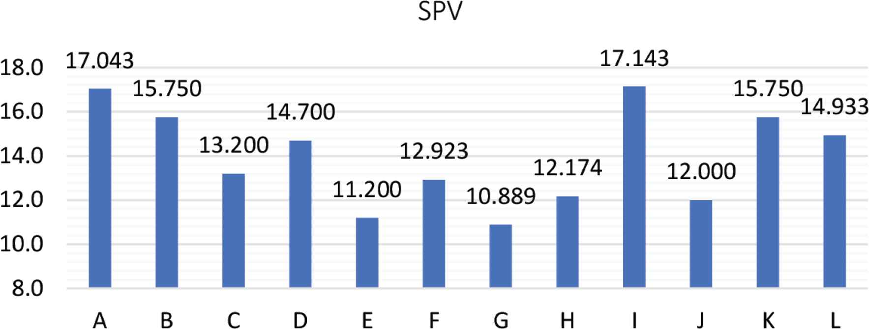
Twelve SPVs for supplier assessment.
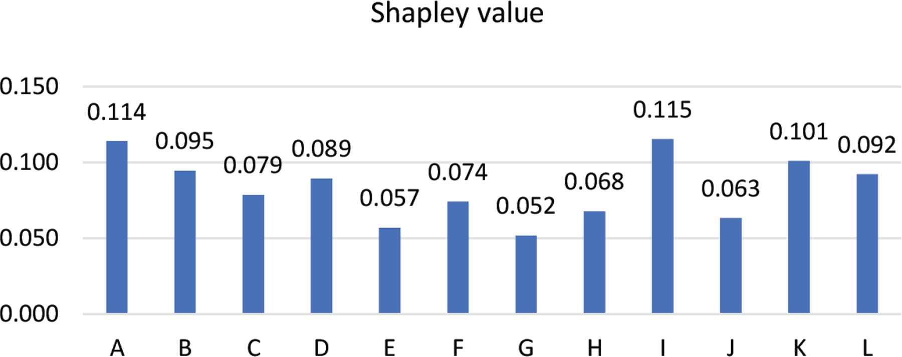
Twelve Shapley values for the manufacturing process of X manufacturer.
4.1. Numerical Analysis of Supplier Assessment
A numerical simulation is conducted to determine whether the SPVs calculated in the first stage of the supplier assessment game are optimal for both the supplier and the manufacturer. We assume that the proposed game is a zero-sum game which exists a mixed-strategy Nash equilibrium. When the supplier and manufacturer choose their mixed Nash equilibrium strategies, the manufacturer’s expected payoff is vi and the supplier’s expected payoff is the negative of vi; see Eq. (7). Equilibrium is reached when the manufacturer, for the given q-mixed strategies, chooses its p-mixed strategies to maximize Eq. (7) (i.e., the manufacturer’s expected payoff). Simultaneously the supplier, for the given p-mixed strategies, chooses its q-mixed strategies to maximize the negative of Eq. (7) (i.e., the supplier’s expected payoff) or to minimize the same equation.
According to Eq. (7), the expected payoff of the manufacturer’s optimal strategies is represented by the SPV. This study presents six cases for validation; see Table 1 and Figure 5a–5f. Each case plays a 2 × 4 payoff matrix game. The “prevent-exploitation method” [27] is applied to find the mixed strategy Nash equilibrium in the 2 × 4 payoff matrix game. In the first case, two mixed strategies are chosen for the manufacturer: services demand (u1) and priority (u1). Two mixed strategies are chosen for the supplier: cost of manufacturing (d2) and delivery performance (d3), and two strategies are deleted: quality of products (d1) and technology of supplier (d4). Thus, this game can be simplified to 2 × 2 payoff matrix. Consider Eq. (7) as a function of all the p-mixed strategies and the q-mixed strategies and draw it in three-dimensional space. The saddle-shaped front and rear cross-sections are valley or U-shaped with the minimum value in the middle, while the lateral cross-section looks like a peak or inverted U-shape with the maximum value in the middle. If the supplier or manufacturer has just two pure strategies, p(u1) and q(d2) can be determined by an integer (1 or 0). If the probability of the manufacturer choosing the first strategy is p(u1), then the probability of choosing the second strategy is p(u2) = 1 − p(u1); if the probability of the supplier choosing the first strategy is q(d2), then the probability of choosing the second strategy is q(d3) = 1 − q(d2). The graph for this supplier assessment game is drawn in three dimensions; see Figure 5a, where the x- and y-axis are on the horizontal plane, and the z-axis points vertically upward. The p(u1) of the manufacturer is shown along the x-axis, the q(d2) of the supplier along the y-axis, and the value v of the expected payoff along the z-axis. A cross-section of the graph along the x direction will show the maximum value of v with respect to p(u1) as a peak. A cross-section along the y direction will show that v is minimized with respect to q(d2), and therefore appears as a valley. Thus, the graph is saddle-shaped, as illustrated in Figure 5a. The mixed strategies N.E. v1 (i.e., SPV) is called a saddle point from which the manufacturer and supplier cannot deviate.
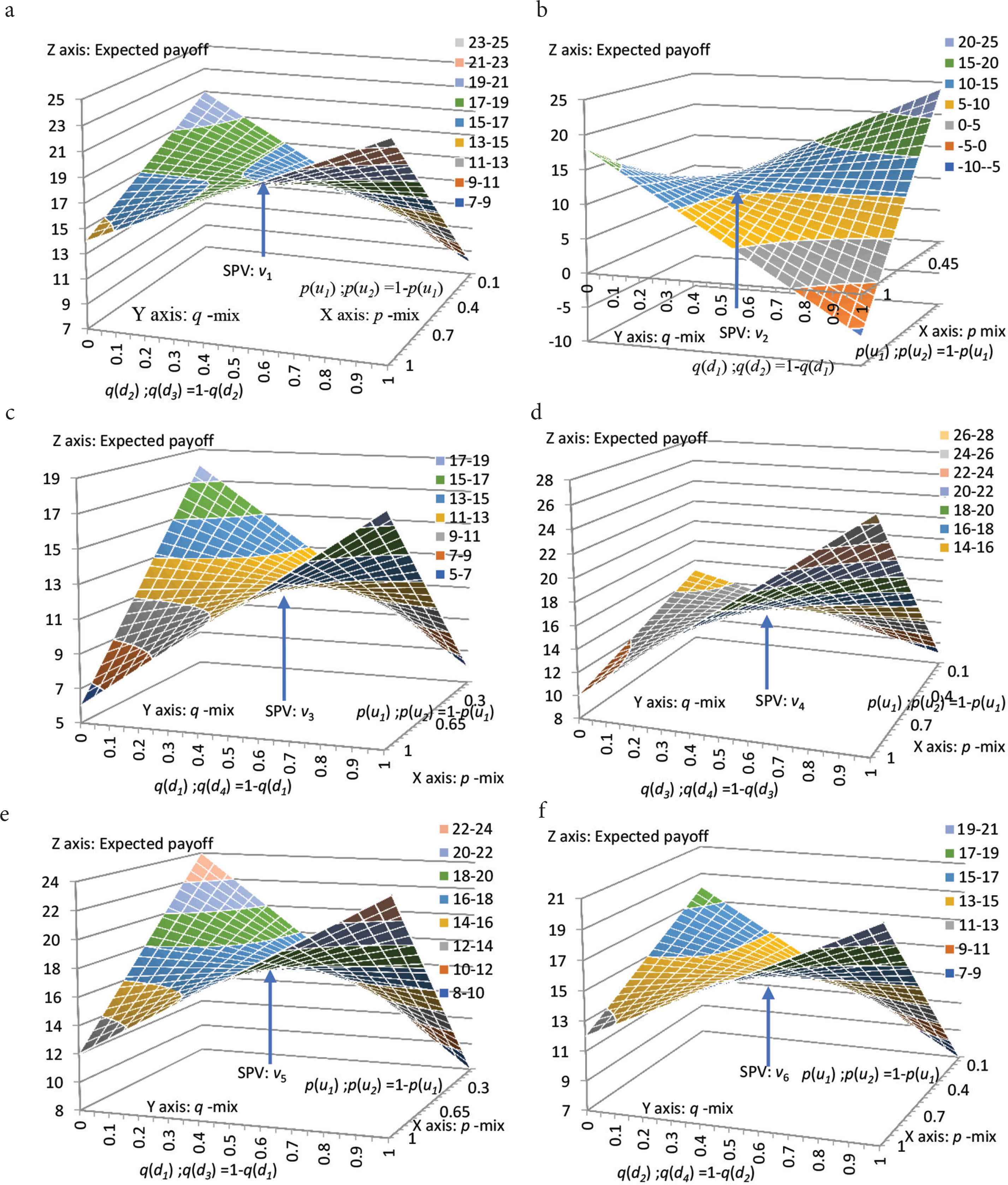
The SPV is represented as a saddle point when the supplier chooses the: (a) cost of manufacturing (d2) and delivery performance (d3) mixed strategy; (b) quality of products (d1) and cost of manufacturing (d2) mixed strategy; (c) quality of products (d1) and the technology of the supplier (d4) mixed strategy; (d) delivery performance (d3) and technology of the supplier (d4) mixed strategy; (e) quality of products (d1) and delivery performance (d3) mixed strategy; (f) cost of manufacturing (d2) and technology of the supplier (d4) mixed strategy.
Similarly, as shown in Figure 5b, in the second case, we also delete two of the manufacturer’s strategies: delivery performance (d3) and technology of the supplier (d4) leaving the two mixed strategies of quality of products (d1) and cost of manufacturing (d2). The numerical simulation shows that the saddle point of this game is the SPV (v2), as shown in Figure 5b. The third case also can be simplified to a 2 × 2 payoff matrix, with the two mixed strategies of quality of products (d1) and technology of the supplier (d4). We find that the saddle point of this game is the SPV (v3); see Figure 5c. The fourth case presents two mixed strategies of delivery performance (d3) and technology of the supplier (d4). The saddle point of this game is the SPV (v4); see Figure 5d. In the fifth and the sixth case, we also find that the saddle point of the game to be the SPV (v5) and the SPV (v6); see Figure 5e and 5f. The value of vi (i.e., SPV) is the mixed strategy N.E., that is, the simultaneous maximum with respect to the expected payoff to the manufacturer and the minimum with respect to the expected payoff for the supplier. This is called the minimax value of the zero-sum game. Thus, this value (i.e., SPV) of the supplier assessment game is optimal for the manufacturer and the supplier. The higher SPV supplier obtains, the higher the expected payoff the manufacturer gains and the more orders manufacturer is willing to give to the supplier in the manufacturing process. The SPV appears to offer useful information concerning the decision-making of supplier assessment.
4.2. Validation of Manufacturing Order Allocation
In this experimental example, the administrator of the SCM is responsible for the deployment of a supplier order budget of 10,000 and provides central management and monitoring with consideration of the majority levels (for the manufacturing process of X manufacturer) for 12 suppliers. His/her goal is to find the most effective allocation of suppliers for the manufacturing process given one majority level. The 12 SPVs are calculated exactly using Eqs. (1)–(7). Figure 3 shows the sequence of the 12 suppliers’ SPVs as an output vector. We use Eq. (8) to obtain the threshold of the majority level mh = 83.85 according to the SPV vector output. Using these threshold values, we apply Eq. (10) to calculate the exact Shapley values for the suppliers as shown in Figure 4 and Table 5. Then, a manufacturing order allocation plan comprised of a minimum set of suppliers for the manufacturing process using Eq. (11); see Table 5.
| Manufacturing process | Supplier | SPVs | Threshold value mh | Shapley value si | Allocation amount for supplier ei |
|---|---|---|---|---|---|
| Manufacturer X | A | 17.043 | mh = 83.85 | 0.114 | 1140.0 |
| B | 15.750 | 0.095 | 945.2 | ||
| C | 13.200 | 0.079 | 786.4 | ||
| D | 14.700 | 0.089 | 894.7 | ||
| E | 11.200 | 0.057 | 570.0 | ||
| F | 12.923 | 0.074 | 743.1 | ||
| G | 10.889 | 0.052 | 519.5 | ||
| H | 12.174 | 0.068 | 678.2 | ||
| I | 17.143 | 0.115 | 1154.4 | ||
| J | 12.000 | 0.063 | 634.9 | ||
| K | 15.750 | 0.101 | 1010.1 | ||
| L | 14.933 | 0.092 | 923.5 | ||
| Total | 167.7 | 1 | 10,000 |
Twelve examples for computing the SPVs, Shapley values, and allocation amount for suppliers
As can be seen in Table 5, from supplier A to L, the higher the SPV, the higher the Shapley value (such as for suppliers A and I). The Shapley value shows the relative importance of the suppliers. Suppliers with a higher Shapley value receive more order quantities than suppliers with a lower Shapley value. In contrast, the lower the SPV value, the lower the Shapley value (as for suppliers E and G), so the fewer order quantities received.
5. CONCLUSION AND FUTURE WORK
In the proposed framework, two game theory models are applied to develop the supply chain decision and analysis process. The first model creates a Nash equilibrium game strategy to find the SPV for each supplier, for optimal supplier assessment. The second model uses the SPVs to compute a Shapley value for each supplier given the majority threshold. The Shapley values are then used to build a rating system for the deployment of suppliers within one manufacturing flow. In this way, we can provide a fair and equitable allocation of a manufacturing order. The simulation results demonstrate the suitability of the two game theory models for the determination of the deployment of suppliers. The experiments help us to demonstrate that the framework connecting the Nash equilibrium and Shapley values, will enable the manufacturer to prioritize their budget for a manufacturing process. The experimental results confirm that the framework can assist managers in assessing manufacturer demands and supplier’s capacities for manufacturing order allocation. In future work, we will use real data to verify the suitability of the proposed framework for the manufacturing flow management process.
CONFLICTS OF INTEREST
The authors declare they have no conflicts of interest.
AUTHORS’ CONTRIBUTION
Both authors designed the model and the computational framework and analyzed the data. All authors discussed the experimental results and contributed to the final manuscript.
ACKNOWLEDGMENTS
The authors appreciate the time and effort of the editors and reviewers in providing constructive comments which have helped to improve the manuscript.
REFERENCES
Cite this article
TY  - JOUR
AU  - Cheng-Kuang Wu
AU  - Yu-Min Chuang
PY  - 2020
DA  - 2020/10/24
TI  - Game Theoretic Strategies for Supplier Capability
Assessment and Manufacturing Order Allocation
JO  - Journal of Risk Analysis and Crisis Response
SP  - 121
EP  - 129
VL  - 10
IS  - 4
SN  - 2210-8505
UR  - https://doi.org/10.2991/jracr.k.201014.002
DO  - 10.2991/jracr.k.201014.002
ID  - Wu2020
ER  -