Journal of Nonlinear Mathematical Physics

Volume 27, Issue 1, October 2019, Pages 130 - 161

Inverse Scattering Transform and Solitons for Square Matrix Nonlinear Schrödinger Equations with Mixed Sign Reductions and Nonzero Boundary Conditions

Authors
Alyssa K. Ortiz1
1Department of Mathematics, University of Colorado Colorado Springs, 1420 Austin Bluffs Pkwy Colorado Springs, Colorado 80918, United States,aortiz@uccs.edu,bprinari@uccs.edu
Barbara Prinari1, 2
2Department of Mathematics, University of Buffalo, 244 Mathematics Building Buffalo, New York 14260, United States,bprinari@buffalo.edu
Received 1 March 2019, Accepted 13 July 2019, Available Online 25 October 2019.
DOI
10.1080/14029251.2020.1683996How to use a DOI?
Keywords
Inverse scattering transform; nonlinear waves; solitons; nonlinear Schrödinger systems
Abstract

The inverse scattering transform (IST) with nonzero boundary conditions at infinity is developed for a class of 2 × 2 matrix nonlinear Schrödinger-type systems whose reductions include two equations that model certain hyperfine spin F = 1 spinor Bose-Einstein condensates, and two novel equations that were recently shown to be integrable, and that have applications in nonlinear optics and four-component fermionic condensates. In our formulation, both the direct and the inverse problems are posed in terms of a suitable uniformization variable which allows us to develop the IST on the standard complex plane instead of a two-sheeted Riemann surface or the cut plane with discontinuities along the cuts. Analyticity, symmetries and asymptotics of the scattering eigenfunctions and scattering data are derived, and properties of the discrete spectrum are analyzed in detail. In addition, the general behavior of the soliton solutions for all four reductions is discussed, and some novel soliton solutions are presented.

Copyright
© 2020 The Authors. Published by Atlantis and Taylor & Francis
Open Access
This is an open access article distributed under the CC BY-NC 4.0 license (http://creativecommons.org/licenses/by-nc/4.0/).

1. Introduction

In the last two decades there has been an increased focus in the study of multicomponent Bose-Einstein condensates (BECs) within the field of atomic and nonlinear wave physics, with a particular emphasis on spinor condensates, i.e., systems whose atoms are in a single hyperfine state but possess internal spin degrees of freedom. Various multicomponent ultracold gases and condensates have been realized experimentally using optical trapping techniques [21].

Spinor BECs formed by atoms with spin F are characterized by a macroscopic wave function with 2F + 1 components, and are associated with various phenomena not present in single-component BECs, such as formation of spin domains, spin textures and topological states. Various types of solitary wave structures (solitons) were first predicted to occur and then observed in focusing and defocusing spinor BECs. These include gap (bright) solitons and dark solitons in optical lattices, polar-core spin vortices, topological states, and topological Wigner crystals of half-solitons. We refer the inquisitive reader to [19, 22, 36] for more details on the experimental examination of spinor BECs.

Many theoretical works have dealt with multicomponent vector solitons in F = 1 spinor BECs, which are characterized by 3-component macroscopic wave functions. In particular, a completely integrable model for homogeneous one-dimensional spin-1 BECs (i.e., a cigar-shaped spin-1 BEC in the absence of external magnetic fields) was proposed by Wadati et al. in [15], and subsequently extended and generalized in [7,1012,16,24,33,40,41] to also include both attractive and repulsive inter-atomic interactions, spin F = 2 condensates, as well as a finite, nonzero background. The generalization to a nonzero background is particularly important for both kinds of nonlinearity (attractive or repulsive), since in this context the BEC can exhibit domain wall solutions [20, 29], dark-bright soliton complexes [3, 18, 27, 28, 30, 43], and in the attractive/focusing case also rogue wave solutions [24, 35].

In [39] Tsuchida showed that the matrix NLS in [15] remains integrable under more general reductions for the matrix potential, and in [34] the Inverse Scattering Transform (IST) was developed for this class of matrix nonlinear Schrödinger type systems, defined as

iQt+Qxx2QRQ=0,R=ΣQΩ,(1.1)
where: Q(x, t) is a 2 × 2 matrix valued potential function; subscripts x, t denote partial derivatives with respect to the spatial variable x and the time variable t, respectively; the matrices Σ and Ω are constant 2 × 2 Hermitian matrices, and Q is the Hermitian conjugate of Q; the matrix potential Q vanishes rapidly enough at space infinity. The purpose of this work is to develop the IST for the above matrix equations with nonzero boundary conditions for Q, R as x → ±∞. As mentioned in [34,39], the system can be simplified by means of linear transformations QU1QU2 with U1, U2 constant, nonsingular matrices, which allows to choose the Hermitian matrices Σ, Ω in canonical form, i.e., diagonal and with diagonal entries equal to 0 or ±1. In order to have a fully coupled system, rather than a triangular one, one can further assume without loss of generality Σ and Ω to be 2 × 2 diagonal matrices with entries equal to ±1. Specifically, let σ3 be the third Pauli matrix, and I2 denote the 2 × 2 identity matrix. Then one has the following four inequivalent reductions for the system (1.1).
  • Case 1 - Defocusing (Σ = I2, Ω = I2):

    itq1+x2q12q1[|q1|2+2|q0|2]2q02q1*=0,(1.2a)
    itq1+x2q12q1[|q1|2+2|q0|2]2q02q1*=0,(1.2b)
    itq0+x2q12q0[|q1|2+|q0|2+|q1|2]2q1q0*q1*=0.(1.2c)

  • Case 2 - Focusing (Σ = I2, Ω = −I2):

    itq1+x2q1+2q1[|q1|2+2|q0|2]+2q02q1*=0,(1.3a)
    itq1+x2q1+2q1[|q1|2+2|q0|2]+2q02q1*=0,(1.3b)
    itq0+x2q1+2q0[|q1|2+|q0|2+|q1|2]+2q1q0*q1*=0.(1.3c)

  • Case 3 - mixed signs (Σ = σ3, Ω = σ3):

    itq1+x2q12q1[|q1|22|q0|2]2q02q1*=0,(1.4a)
    itq1+x2q12q1[|q1|22|q0|2]2q02q1*=0,(1.4b)
    itq0+x2q12q0[|q1|2|q0|2+|q1|2]+2q1q0*q1*=0.(1.4c)

  • Case 4 - mixed signs (Σ = σ3, Ω = −σ3):

    itq1+x2q1+2q1[|q1|22|q0|2]+2q02q1*=0,(1.5a)
    itq1+x2q1+2q1[|q1|22|q0|2]+2q02q1*=0,(1.5b)
    itq0+x2q1+2q0[|q1|2|q0|2+|q1|2]2q1q0*q1*=0.(1.5c)

Cases 1 and 2 with nonzero boundary conditions have been considered in various previous works [16, 33, 40], whereas cases 3 and 4 with nonzero boundary conditions are novel. In this work, we will cover all four cases, showing that the results for cases 1 and 2 can be recovered as a byproduct.

It is worth pointing out that cases 3 and 4 correspond to a “mixed sign” case for coupled NLS systems where the nonlinearity in the norm is of Minkowski-type instead of the Euclidean-type norm that appears in cases 1 and 2. Soliton solutions for the mixed sign vector NLS have been found with both zero and nonzero boundary conditions in [9,17,31,38,42]. In the two-component case, the “mixed sign” NLS models the dynamics of vector solitons in waveguide arrays. The “mixed sign” two-component coupled NLS can also be used to model a series of drops of a binary BEC trapped in an optical lattice. However, the matrix coupled situation is different. The signs of the coupling constants now correspond to s-wave scattering lengths accounting for interspecies and intraspecies atomic interactions of the condensates. Therefore, unlike cases 1 and 2, the PDEs in cases 3 and 4 cannot physically model three-component F = 1 BECs. Nevertheless, they can model two classes of physical problems, nonlinear optics and four-component fermionic condensates. The interested reader can find more details in references [13, 14, 34] concerning cases 3 and 4 in the context of nonlinear optics. We refer the reader to references [25, 34] for more information regarding cases 3 and 4 in the context of four-component fermionic condensates.

In the following, the matrix potential Q(x, t) is chosen to be a symmetric matrix:

Q(x,t)=(q1(x,t)q0(x,t)q0(x,t)q1(x,t)).(1.6)

Note that we could have also considered the off-diagonal entries to be q0(x, t) and −q0(x, t), but by performing a change of variables on each diagonal component, i.e. qj → −qj for j = ±1, one can easily check that the same equations as in the symmetric case are recovered. Note also that if one is interested in four-component fermionic condensates, Q(x, t) is not necessarily symmetric, and the corresponding results can be obtained by disregarding the second symmetry (see Sec. 2.4).

In order for the system (1.1) to allow for constant nonzero boundary conditions as x → ±∞, one can perform a simple gauge transformation Q(x,t)=Q^(x,t)e2ik02t, where k0 is a real positive constant. Dropping the ^ for simplicity, the equation then becomes

iQt+Qxx2(QRνk02I2)Q=0,(1.7)
where ν = 1 in cases 1 and 3, and ν = −1 in cases 2 and 4. We will then consider the system (1.7) under constant nonzero boundary conditions (NZBC):
Q(x,t)Q±asx+.(1.8)

Assuming that for constant NZBC the derivative terms iQt and Qxx also vanish in the limit x → ±∞, the following constraints are imposed on the NZBC:

R±Q±=Q±R±=νk02I2,(1.9)
which are consistent with (1.7), they are time-independent, and are amenable to simple treatment by IST. If we look at each individual component of the matrix Q±, we get the following equivalent set of constraints for cases 1 and 2:
|q1,±|2=|q1,±|2,|q0,±|2=k02|q1,±|2=k02|q1,±|2,q1,±q0,±*+q0,±q1,±*=0,(1.10)
and for cases 3 and 4:
|q1,±|2=|q1,±|2,|q0,±|2=|q1,±|2k02=|q1,±|2k02,q1,±q0,±*q0,±q1,±*=0.(1.11)

The paper is organized as follows. Section 2 covers the direct scattering problem for Eq. (1.7). In Section 3 we develop the inverse scattering problem for the eigenfunctions as a Riemann-Hilbert problem (RHP) with poles. We solve the RHP in the case of simple poles and reconstruct the potential in terms of the eigenfunctions and scattering data. In Section 4 we focus on reflectionless potentials, i.e. pure soliton solutions and include several plots to illustrate the distinguished features of the various solutions. In Section 5 we provide some concluding remarks.

2. Direct Scattering

2.1. Lax Pair, Riemann Surface and Uniformization Coordinate

The MNLS equation (1.7) for a 2 × 2 potential matrix Q(x, t) can be recovered as the compatibility condition (ϕxt = ϕtx) of the Lax pair:

φx=Uφ,φt=Vφ,(2.1)
with
U(x,t,k)=ikσ_3+Q_,V(x,t,k)=2ik2σ_3+2kQ_+iσ_3[Q_x+νk02I4Q_2],(2.2a)
σ_3=(I20202I2),Q_=(02QR02),(2.2b)
where I2, I4 and 02 are the 2 × 2 identity matrix, 4 × 4 identity matrix and 2 × 2 zero matrix respectively. In the usual manner, we will henceforth refer to the first equation of the Lax pair (2.1) as the scattering problem.

It is useful to note for future reference that Q_ and σ_3 anticommute, namely

Q_σ_3=σ_3Q_.(2.3)

Taking into account the boundary conditions (1.8), asymptotically the scattering problem becomes

φx=U±φ,U±=ikσ_3+Q_±,withQ_±=(02Q±R±02).(2.4)

It is useful to note that there is an equivalent 4 × 4 constraint to the 2 × 2 constraint (1.9) on the NZBC (1.8)

R±Q±=Q±R±=νk02I2,Q±2=νk02I4.(2.5)

The eigenvalues of U± are λ=±ik2νk02, where each eigenvalue has a multiplicity of 2. We need to account for the multivaluedness/branching of these eigenvalues, which we will accomplish by introducing a two-sheeted Riemann surface

λ=k2νk02,(2.6)
such that λ(k) is a single-valued on this surface. The branch points correspond to λ2 = 0, namely k=±νk0. We note that the branch points are k = ±k0 for cases 1 and 3, and k = ±ik0 for cases 2 and 4.

For cases 1 and 3, let us introduce

kk0=r1eiθ1onI,(2.7a)
k+k0=r2eiθ2onII,(2.7b)
where ℂI denotes the first sheet of the Riemann surface and ℂII denotes the second sheet. We can then define λ(k) on the two Riemann sheets in polar coordinates as
λ(k)=r1r2ei(θ1+θ2)/2onI,(2.8a)
λ(k)=r1r2ei(θ1+θ2)/2onII,(2.8b)
so that choosing 0 ≤ θ1 < 2π and −πθ2 < π places the discontinuities of λ(k) on the real k-axis for k ∈ (−∞, −k0) ∪ (k0, ∞). The Riemann surface is then obtained by gluing the upper branch cut (k0, ∞) of ℂI to the lower branch cut (−∞, −k0) of ℂII, and vice versa, so that λ(k) is now continuous on the entire Riemann surface, including across the branch cut.

Similarly for cases 2 and 4, we introduce

k+ik0=r1eiθ1onI,(2.9a)
kik0=r2eiθ2onII,(2.9b)
and define λ(k) on the two copies of the complex plane as
λ(k)=r1r2ei(θ1+θ2)/2onI,(2.10a)
λ(k)=r1r2ei(θ1+θ2)/2onII,(2.10b)
so that choosing −π/2 ≤ θj < 3π/2 for j = 1, 2 places the branch cut on the imaginary k-axis for ki[−k0, k0]. We again form the Riemann surface by gluing the two sheets ℂI and ℂII together along the cut, which makes and make λ(k) continuous across the branch cut i[−k0, k0].

We will follow the same strategy as in [4, 6, 8, 32] by introducing a uniformization variable

z=k+λ,(2.11)
where the inverse transformation is
k=12(z+νk02/z),λ=12(zνk02/z).(2.12)

Using these definitions of z, k and λ, we observe that in cases 1 and 3, the branch cuts of both copies of the complex plane are mapped onto the real z-axis. The first Riemann sheet ℂI is mapped onto the upper half of the complex z-plane and the second Riemann sheet ℂII is mapped onto the lower half plane of the complex z-plane. A neighborhood of k = ∞ on both sheets is mapped onto either a neighborhood of z = 0 or z = ∞ depending on the sign of Imk (cf. Fig. 1).

Fig. 1:

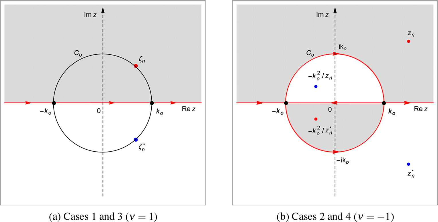
Left/Right: The complex z-plane, showing the regions D± where Imλ > 0 (gray) and Imλ < 0 (white), respectively. Also shown in the figures are the oriented contours for the Riemann-Hilbert problem (red), and the symmetries of the discrete spectrum of the scattering problem.

In cases 2 and 4, we observe that the branch cut on both Riemann sheets is mapped onto the circle C0 centered at z = 0 with radius k0 in the complex z-plane, i.e.

C0={z:|z|=k0}.(2.13)

The first Riemann sheet ℂI is mapped onto the exterior of C0, and the second Riemann sheet ℂII is mapped onto the interior of C0. Moreover, z(∞I) = ∞ and z(∞II) = 0, where ∞I signifies that k → ∞ on ℂI, and ∞II denotes that k → ∞ on ℂII (cf. Fig. 1).

Consequently, for cases 1 and 3, Imλ > 0 corresponds to the region D in the z-plane, and Imλ < 0 corresponds to the region D in the z-plane, where

ν=1:D+={z:Imz>0},D={z:Imz<0}.(2.14)

Similarly, for cases 2 and 4, Imλ > 0 corresponds to D+ and Imλ < 0 corresponds to D such that

ν=1:D+={z:(|z|2k02)Imz>0},D={z:(|z|2k02)Imz<0}.(2.15)

The regions D+ and D are represented in Figure 1, where D+ is depicted as the gray region and D is depicted as the white region. For cases 1 and 3, we observe that D+ is the UHP of the z-plane and D is the LHP of the z-plane. For cases 2 and 4, we observe that the region D+ includes the exterior of C0 in the upper-half z-plane and the interior of C0 in the lower-half z-plane. Conversely, the region D includes the interior of C0 in the upper-half z-plane and the exterior of C0 in the lower-half z-plane.

We will show in the next section that the sign of Imλ determines the region of analyticity of the Jost eigenfunctions. From now on, it will be more convenient to express all k dependence as z dependence where appropriate.

2.2. Jost Solutions and Analyticity

The Jost solutions are defined as the asymptotic eigenvector solutions of the asymptotic scattering problem (2.4). We can write the asymptotic eigenvector matrix as

X±(k)=I2ik+λσ_3Q_±I2izσ_3Q_±,(2.16)
such that
U±X±=iλX±σ_3.(2.17)

We observe that

detX±(z)=(2λλ+k)2=(γ(z))2,γ(z)=1νk02z2,(2.18a)
X±1(z)=1γ(z)(I2+izσ_3Q_±),(2.18b)
where the inverse matrices X±1 are defined for values of z where γ(z) ≠ 0, i.e. away from the branch points: z ≠ ±k0 in cases 1 and 3 (ν = 1), and z ≠ ±ik0 in cases 2 and 4 (ν = −1).

We will now consider the time dependence of the eigenfunctions. The time evolution of the eigenfunctions is dictated by the second equation in (2.1), which asymptotically as x → ±∞ yields ϕt = V±ϕ with V±=2ik2σ_3+2kQ_±, taking into account the boundary conditions (1.8), the constraint (2.5), and the fact that Q_x02 as x → ±∞. One can easily verify that

V±X±=2ikλX±σ_3,(2.19)
noting that 2kλ=(z2k04/z2)/2. Therefore the eigenvector matrix X± is a simultaneous asymptotic solution of both equations in the Lax pair.

We then define the Jost solutions as the

Φ(x,t,z)(ϕ(x,t,z),ϕ¯(x,t,z))=X(z)eiθ(x,t,z)σ_3+(1)asx,(2.20a)
Ψ(x,t,z)(ψ¯(x,t,z),ψ(x,t,z))=X+(z)eiθ(x,t,z)σ_3+(1)asx,(2.20b)
where
θ(x,t,z)λ(z)(x+2k(z)t),(2.21)
and φ(x, t, z), ϕ¯(x,t,z), ψ¯(x,t,z) and ψ(x, t, z) are 4 × 2 matrices. It is also useful to note the asymptotic behavior of Φ(x, t, z) and Ψ(x, t, z) for each 2 × 2 block:
ϕ(x,t,z)(I2izR)eiθ(x,t,z)asx,(2.22a)
ϕ¯(x,t,z)(izQI2)eiθ(x,t,z)asx,(2.22b)
ψ¯(x,t,z)(I2izR+)eiθ(x,t,z)asx+,(2.22c)
ψ(x,t,z)(izQ+I2)eiθ(x,t,z)asx+.(2.22d)

As usual, the continuous spectrum of the scattering problem corresponds to values of (k, λ), or, equivalently, z, such that the all four eigenfunctions above are bounded for all x ∈ ℝ, which requires λ(k) ∈ ℝ. Correspondingly, we denote the continuous spectrum in k as Σk = ℝ \ [−k0, k0] for cases 1 and 3 (ν = 1), and Σk = ℝ ∪ i(−k0, k0) for cases 2 and 4 (ν = −1). In the z-plane, the continuous spectrum is Σz = ℝ for ν = 1 and Σz = ℝ ∪ C0 for ν = −1.

It is convenient to define modified eigenfunctions related to these Jost solutions (2.20a), (2.20b) that have simpler asymptotic behavior as x → ±∞:

(x,t,z)(M(x,t,z),M¯(x,t,z))=Φ(x,t,z)eiθ(x,t,z)σ_3,(2.23a)
𝒩(x,t,z)(N¯(x,t,z),N(x,t,z))=Ψ(x,t,z)eiθ(x,t,z)σ_3,(2.23b)
such that
limx(x,t,z)=limxΦ(x,t,z)eiθ(x,t,z)σ_3=X,zΣz,(2.24a)
limx𝒩(x,t,z)=limxΨ(x,t,z)eiθ(x,t,z)σ_3=X+,zΣz.(2.24b)

Following the same strategy as in [4], one can express the modified eigenfunctions M, M¯, N, N¯ as solutions of suitable Volterra-type integral equations, and show that under some mild integrability conditions of Q(x, t) − Q± for x ∈ (xo, ∓∞) and any fixed t ≥ 0, the modified eigenfunctions M(x, t, z) and N(x, t, z) can be analytically extended to D+ in the z-plane. Similarly, the modified eigenfunctions M¯(x,t,z) and N¯(x,t,z) can be analytically extended to D+ in the z-plane.

2.3. Scattering Coefficients

Using Jacobi’s formula, we conclude that any solution ϕ(x, t, z) of (2.1) satisfies x(detϕ) = t(detϕ) = 0 since U and V are traceless. Then it follows from (2.24a) and (2.24b) that

detΦ(x,t,z)=detΨ(x,t,z)=detX±=(γ(z))2,x,t,zΣz.(2.25)

Therefore, for all zΣ0:=Σ\{±νk0}, Φ and Ψ are both fundamental solutions of the scattering problem. Hence there exists a proportionality matrix S(z) between the two fundamental solutions, such that

Φ(x,t,z)=Ψ(x,t,z)S(z),S(z)=(a(z)b¯(z)b(z)a¯(z)),x,t,zΣ0,(2.26)
where S(z) is referred to as the scattering coefficient matrix. Column-wise, (2.26) can be expressed by
ϕ=ψb+ψ¯a,ϕ¯=ψa¯+ψ¯b¯,(2.27)
where a, b, ā, b¯ are the 2 × 2 block matrices of the scattering coefficient matrix S(z). Since Φ and Ψ are both simultaneous solutions of (2.1), the scattering coefficients are independent of both x and t. Furthermore, (2.25) and (2.26) imply that detS(z) = 1. In turn, from (2.27) it also follows that:
deta(z)=Wr(ϕ,ψ)/Wr(ψ¯,ψ)det(ϕ,ψ)/detΨ=det(ϕ,ψ)/(γ(z))2,(2.28a)
deta¯(z)=Wr(ψ¯,ϕ¯)/Wr(ψ¯,ψ)det(ψ¯,ϕ¯)/detΨ=det(ψ¯,ϕ¯)/(γ(z))2,(2.28b)
where Wr(u, v) denotes the Wronskian determinant of 4 × 2 vector functions u and v. In the scalar case, one can show that a(z) can be analytically extended to D+, and ā(z) in D. In the matrix case, (2.28a) and (2.28b) only imply that deta(z) can be analytically extended to D+, and detā(z) can be analytically extended to D. However, following the same strategy outlined in [6, 8, 33], which makes use of the integral equations for the modified eigenfunctions, one can obtain an integral representation for the scattering coefficient matrix which allows to establish analyticity of the 2 × 2 block a(z) to D+, and of ā(z) can be analytically extended to D. Note that it is also possible to establish the analyticity of a(z) and ā(z) using the symmetries of the scattering data, which will be shown in Section 2.4.

We observe that the matrices X±(z) are singular at the branch points z=±νk0, where (2.18b) implies that X±1(z) have simple poles at the branch points. Consequently, in general the scattering coefficients a(z), ā(z), b(z), b¯(z) also have simple poles at the branch points. The behavior of the scattering coefficients at the branch points will be discussed in Section 2.4.

Lastly, for z ∈ Σ0, (2.23a), (2.23b), and (2.27) imply that

M(x,t,z)a1(z)=N¯(x,t,z)+e2iθ(x,t,z)N(x,t,z)ρ(z),(2.29a)
M¯(x,t,z)a¯1(z)=N(x,t,z)+e2iθ(x,t,z)N¯(x,t,z)ρ¯(z),(2.29b)
where we observe that M(x, t, z)a−1(z) is meromorphic in D+, M¯(x,t,z)a¯1(z) is meromorphic in D, and ρ(z), ρ¯(z) are the reflection coefficients defined as
ρ(z)=b(z)a1(z),ρ¯(z)=b¯(z)a¯1(z),zΣ0,(2.30)
and Σ0 is as introduced after Eq. (2.25).

2.4. Symmetries

When an initial-value problem (IVP) is solved using IST, symmetries in the potential lead to symmetries in the Jost solutions, which lead to symmetries in the scattering data. In the case of zero boundary conditions (ZBC), there are two symmetries in the scattering data that follow the symmetries in the potential: (i) R = ΣQΩ; and (ii) Q = QT. With respect to the uniformization variable z, R = ΣQΩ corresponds to zz* ⇔ (k, λ) → (k*, λ*), which we will refer to as the first symmetry (conjugation symmetry on same sheet). The fact that the potential is assumed to be symmetric, i.e. Q = QT, will be referred to as the third symmetry (transpose symmetry).

In the case of NZBC, things are a little more complicated since λ(k) changes sign from one Riemann sheet to another, namely λII(k) = −λI(k). In terms of the uniformization variable, this corresponds to zνk02/z, which reflects the fact that the z-plane is a double covering of the Riemann surface for (k, λ), and which does not arise in the case of ZBC. This additional symmetry will be referred to as the second symmetry (symmetry across sheets). For the remainder of Section 2.4, we will discuss in detail how all three symmetries affect both the eigenfunctions and the scattering data.

2.4.1. First Symmetry: (k, λ) → (k*λ*)

Let us introduce for z ∈ Σz the bilinear combinations

f(x,t,z)=Φ(x,t,z*)JvΦ(x,t,z),g(x,t,z)=Ψ(x,t,z*)JνΨ(x,t,z),(2.31)
where
Jν=(Ω10202Σ).(2.32)

Since Φ and Ψ are both solutions of the scattering problem in (2.1), it can be easily verified that fx = ft = gx = gt = 0, i.e. f, g are independent of x and t. If we evaluate limx→±∞ f(x, t, z) and limx→±∞ g(x, t, z), we obtain the following relations:

Φ(x,t,z*)JνΦ(x,t,z)=Ψ(x,t,z*)JνΨ(x,t,z)=γ(z)Jν,(2.33)
implying
Φ1(x,t,z)=1γ(z)JνΦ(x,t,z*)Jν,Ψ1(x,t,z)1γ(z)JνΨ*(x,t,z*)Jν.(2.34)

We can then solve (2.26) to obtain:

S(z)=Ψ1(x,t,z)Φ(x,t,z)1γ(z)JνΨ(x,t,z*)JνΦ(x,t,z).(2.35)

We will use the following notation to denote the 2 × 2 blocks of the eigenfunction matrices Φ and Ψ:

Φ(x,t,z)=(ϕupϕ¯upϕdnϕ¯dn),Ψ(x,t,z)=(ψ¯upψupψ¯dnψdn).(2.36)

We can then write the relation (2.35) in terms of each 2 × 2 block:

γ(z)a(z)=Ω1ψ¯up(z*)Ω1ϕup(z)Ω1ψ¯dn(z*)Σϕdn(z),(2.37a)
γ(z)a¯(z)=Σψdn(z*)Σϕ¯dn(z)Σψup(z*)Ω1ϕ¯up(z),(2.37b)
γ(z)b(z)=Σψdn(z*)Σϕdn(z)Σψup(z*)Ω1ϕup(z),(2.37c)
γ(z)b¯(z)=Ω1ψ¯up(z*)Ω1ϕ¯up(z)Ω1ψ¯dn(z*)Σϕ¯dn(z),(2.37d)
where the x, t dependence of the eigenfunctions on the right-hand side has been omitted for shortness. The relations above provide an alternative way to show that a(z) can be analytically extended to D+ and ā(z) can be analytically extended to D, on account of the corresponding analyticity properties of the eigenfunctions in terms of which they are expressed.

It follows from the analog of Theorem 2.4 in [33] that γ(z)S(z) with γ(z) defined in (2.18a) is continuous for all z ∈ Σz, including the branch points. However, as stated earlier, the 2×2 scattering coefficients a(z), ā(z), b(z), b¯(z) in general have simple poles at the branch points z=±νk0, with

Resz=±k0a(z)=±k02[Ω1ψ¯up(x,t,±k0)Ω1ϕup(x,t,±k0)Ω1ψ¯dn(x,t,±k0)Σϕdn(x,t,±k0)],(2.38a)
Resz=±k0a¯(z)=±k02[Σψdn(x,t,±k0)Σϕ¯dn(x,t,±k0)Σψup(x,t,±k0)Ω1ϕ¯up(x,t,±k0)],(2.38b)
limz±k0(zk0)b(z)=±k02[Σψdn(x,t,±k0)Σϕdn(x,t,±k0)Σψup(x,t,±k0)Ω1ϕup(x,t,±k0)],(2.38c)
limz±k0(zk0)b¯(z)=±k02[Ω1ψ¯up(x,t,±k0)Ω1ϕup(x,t,±k0)Ω1ψ¯dn(x,t,±k0)Σϕdn(x,t,±k0)],(2.38d)
for cases 1 and 3 (ν = 1), and
Resz=±ik0a(z)=±ik02[Ω1ψ¯up(x,t,ik0)Ω1ϕup(x,t,±ik0)Ω1ψ¯dn(x,t,ik0)Σϕdn(x,t,±ik0)],(2.39a)
Resz=±ik0a¯(z)=±ik02[Σψdn(x,t,ik0)Σϕ¯dn(x,t,±ik0)Σψup(x,t,ik0)Ω1ϕ¯up(x,t,±ik0)],(2.39b)
limz±ik0(zik0)b(z)=±ik02[Σψdn(x,t,ik0)Σϕdn(x,t,±ik0)Σψup(x,t,ik0)Ω1ϕup(x,t,±ik0)],(2.39c)
limz±ik0(zik0)b¯(z)=±ik02[Ω1ψ¯up(x,t,ik0)Ω1ϕup(x,t,±ik0)Ω1ψ¯dn(x,t,ik0)Σϕdn(x,t,±ik0)],(2.39d)
for cases 2 and 4 (ν = −1). Furthermore, we observe that if deta(z) ≠ 0, detā(z) ≠ 0 for z ∈ Σz, the reflection coefficients ρ(z) and ρ¯(z) both have a removable singularity at the branch points and so they are defined for all z ∈ Σz. Consequently, the equations (2.29a) can also be considered for all z ∈ Σz.

If we examine the 2 × 2 blocks of (2.33), we find the following conjugation symmetries for Φ(z):

ϕup(z*)Ω1ϕup(z)ϕdn(z*)Σϕdn(z)=γ(z)Ω1,(2.40a)
ϕup(z*)Ω1ϕ¯up(z)ϕdn(z*)Σϕ¯dn(z)=02,(2.40b)
ϕ¯up(z*)Ω1ϕup(z)ϕ¯dn(z*)Σϕdn(z)=02,(2.40c)
ϕ¯up(z*)Ω1ϕ¯up(z)ϕ¯dn(z*)Σϕ¯dn(z)=γ(z)Σ,(2.40d)
and similar conjugation symmetries for the 2 × 2 blocks of the eigenfunction matrix Ψ:
ψ¯up(z*)Ω1ψ¯up(z)ψ¯dn(z*)Σψ¯dn(z)=γ(z)Ω1,(2.41a)
ψ¯up(z*)Ω1ψup(z)ψ¯dn(z*)Σψdn(z)=02,(2.41b)
ψup(z*)Ω1ψ¯up(z)ψdn(z*)Σψ¯dn(z)=02,(2.41c)
ψup(z*)Ω1ψup(z)ψdn(z*)Σψdn(z)=γ(z)Σ.(2.41d)

The relation (2.33) also implies that:

S(z*)JνS(z)=Jν,zΣz.(2.42)

If we then consider Eq. (2.42) block by block, we find the corresponding conjugation symmetries for the scattering coefficients:

a(z*)Ω1a(z)b(z*)Σb(z)=Ω1,(2.43a)
a(z*)Ω1b¯(z)b(z*)Σa¯(z)=02,(2.43b)
b¯(z*)Ω1a(z)a¯(z*)Σb(z)=02,(2.43c)
b¯(z*)Ω1b¯(z)a¯(z*)Σa¯(z)=Σ.(2.43d)

The reflection coefficients (2.30) then satisfy the conjugation symmetry

ρ¯(z)=Ω1ρ(z*)Σ1,(2.44)
where we have used the fact that Ω = Ω−1 and Σ = Σ−1. We also observe that
a(z)Ωa(z*)=[Ω1ρ(z*)Σρ(z)]1,a¯(z)Σ1a¯(z*)=[Σρ¯(z*)Ω1ρ¯(z)]1.(2.45)

It follows from (2.42) that

S1(z)=JνS(z)Jν,S1(z)=(c¯(z)d(z)d¯(z)c(z)).(2.46)
which provides a relationship between the 2 × 2 blocks of S(z) and the 2 × 2 blocks of S−1:
c¯(z)=Ω1a(z*)Ω1,(2.47a)
d(z)=Ω1b(z*)Σ,(2.47b)
d¯(z)=Σb¯(z*)Ω1,(2.47c)
c(z)=Σa¯(z*)Σ.(2.47d)

The analogues of (2.28a) and (2.28b) for Ψ(x, t, z) = Φ(x, t, z)S−1(z) are

detc(z)=Wr(ϕ,ψ)/Wr(ϕ,ϕ¯)det(ϕ,ψ)/(γ(z))2,(2.48a)
detc¯(z)=Wr(ψ¯,ϕ¯)/Wr(ϕ,ϕ¯)det(ψ¯,ϕ¯)/(γ(z))2,(2.48b)
which allows us to conclude that
detc(z)=deta(z)forzD+,detc¯(z)=deta¯(z)forzD.(2.49)

Taking into account (2.48a) and (2.48b) we finally obtain the following relations:

deta(z)=deta¯(z*)(deta¯(z*))*,zD+,(2.50a)
deta¯(z)=deta(z*)(deta(z*))*,zD.(2.50b)

2.4.2. Second Symmetry: (k, λ) → (k, −λ)

As mentioned above, the second symmetry relates values of eigenfunctions and scattering data from one Riemann sheet to the other. In terms of the uniformization variable:

(k,λ)(k,λ)zνk02z,(2.51)
which follows from the definitions of λ and z in (2.12). Applying the symmetry zνk02/z to the matrices X± we find the following relation:
X±(z)=izX±(νk02z)σ_3Q_±.(2.52)

If we take into account that θ(νk02/z)=θ(z) and Q_±eiθ(z)σ_3=eiθ(z)σ_3Q_±, which is a direct consequence of (2.3), we get

Φ(x,t,z)=izΦ(x,t,νk02/z)σ_3Q_,Ψ(x,t,z)=izΨ(x,t,νk02/z)σ_3Q_+,zΣz.(2.53)

Explicitly, each 4 × 2 column satisfies

ϕ(x,t,z)=izϕ¯(x,t,νk02/z)R,ϕ¯(x,t,z)=izϕ(x,t,νk02/z)Q,(2.54a)
ψ¯(x,t,z)=izψ(x,t,νk02/z)R+,ψ(x,t,z)=izψ¯(x,t,νk02/z)Q+,(2.54b)

Moreover, from (2.26) and (2.53) it follows that for all z ∈ Σz:

S(νk02/z)=σ_3Q_+S(z)Q_1σ_3νk02σ_3Q_+S(z)Q_σ_3,(2.55)
where we use the fact that Q_±1=νQ_±/k02 to achieve the last equality. If we then examine these results for each 2 × 2 block, we obtain
a(νk02/z)=νk02Q+a¯(z)R,a¯(νk02/z)=νk02R+a(z)Q,(2.56a)
b(νk02/z)=νk02R+b¯(z)R,b¯(νk02/z)=νk02Q+b(z)Q.(2.56b)

Finally, the above relations imply the corresponding symmetries for the reflection coefficients:

ρ(νk02/z)=R+ρ¯(z)Q+1νk02R+ρ¯(z)R+forallzΣz,(2.57a)
ρ¯(νk02/z)=Q+ρ(z)R+1νk02Q+ρ(z)Q+forallzΣz.(2.57b)

Even though the symmetries (2.57a) and (2.57b) are only valid for z ∈ Σz, whenever the specific columns and scattering coefficients involved are analytic, they can be extended to the appropriate regions of the z-plane using the Schwarz reflection principle. We also note that in cases 2 and 4, even the symmetries of the non-analytic scattering coefficients involve the map zz*. This is because unlike what happens in cases 1 and 3, the continuous spectrum is not just a subset of the real z-axis.

2.4.3. Third Symmetry: Q → QT

The third symmetry follows from the fact that we assume the potential Q(x, t) to be a symmetric matrix. We observe the following equivalent relation in terms of Q_:

Q=QTQ_=σ_2Q_Tσ_2,whereσ_2=(02iI2iI202).(2.58)

Proceeding similarly as in the first symmetry, we define

f˜(x,t,z)=ΦT(x,t,z)σ_2Φ(x,t,z),g˜(x,t,z)=ΨT(x,t,z)σ_2Ψ(x,t,z).(2.59)

One can verify that f˜ and g˜ are both independent of x as follows:

xf˜=ΦT[ikσ_3σ_2+Q_Tσ_2ikσ_2σ_3+σ_2Q_]Φ=02,(2.60)
since σ_3σ_2=σ_2σ_3 and Q_Tσ_2=σ_2Q_. A similar result holds for g˜. Evaluating the limits as x → ±∞ we obtain
ΦT(x,t,z)σ_2Φ(x,t,z)=ΨT(x,t,z)σ_2Ψ(x,t,z)=γ(z)σ_2,(2.61)
which implies that
ST(z)σ_2S(z)=σ_2,zΣz.(2.62)

In terms of the 2 × 2 blocks the above symmetry reads:

bT(z)a(z)=aT(z)b(z),a¯T(z)b¯(z)=b¯T(z)a¯(z),(2.63a)
aT(z)a¯(z)bT(z)b¯(z)=I2,a¯T(z)a(z)b¯T(z)b(z)=I2.(2.63b)

The first two relations imply that

ρT(z)=ρ(z),ρ¯T(z)=ρ¯(z),(2.64)
which shows that the reflection coefficients must be symmetric. We also obtain from the last relations the following identities:
a(z)a¯T(z)=[I2ρ¯(z)ρ(z)]1,a¯(z)aT(z)=[I2ρ(z)ρ¯(z)]1,(2.65)
where we have used the (2.64) symmetry relation. It follows from (2.62) that S1(z)σ_2ST(z)σ_2 for z ∈ Σz. Examining the 2 × 2 blocks of this relation gives the following results:
c(z)=aT(z),c¯(z)=a¯T(z),d(z)=b˜T(z),d¯(z)=bT(z).(2.66)

Finally, if we combine this result with (2.47a), (2.47b), (2.47c) and (2.47d) we get

a¯(z)=Ω1a*(z*)Ω1,b¯(z)=Σb*(z*)Ω1,zΣz,(2.67)
which gives a similar relation for the reflection coefficient,
ρ¯(z)=Σρ*(z*)Ω,zΣz.(2.68)

2.5. Discrete Spectrum and Residue Conditions

The discrete spectrum is the set of all values z ∈ ℂ \ Σz where the scattering problem allows eigenfunctions in L2(ℝ). We will show below that these values are the zeros of deta(z) in D+ and the zeros of detā(z) in D. In general, one cannot exclude the possibility of spectral singularities, i.e., zeros that occur on the continuous spectrum Σz. This is a highly nontrivial issue even in the case of zero boundary conditions (see [44]), and to the best of our knowledge no result is currently available in the literature regarding the location of spectral singularities (or sufficient constraints on the potential for their absence) in the case of nonzero boundary conditions. In the following we will assume that deta(z) ≠ 0 and detā(z) ≠ 0 for all z ∈ Σz.

If deta(z) = 0 at a discrete eigenvalue z = zn then the eigenfunctions φ(x, t, zn) and ψ(x, t, zn) become linearly dependent, which can be expressed in general as:

ϕ(x,t,zn)ηn=ψ(x,t,zn)ξn,znD+,(2.69)
for some nonzero complex vectors ξn, ηn ∈ ℂ \ {0}. We note that such vectors are not uniquely defined. Due to the first symmetry, we have a corresponding discrete eigenvalue zn*D such that deta¯(zn*)=0, which produces a linear dependence for the eigenfunctions in D as follows:
ϕ¯(x,t,zn*)η¯n=ψ¯(x,t,zn*)ξ¯n,zn*D,(2.70)
for some nonzero complex vectors ξ¯n, η¯n\{0}. If we assume that ranka(zn) = 0, then deta(z) has a double zero at z = zn and we can make a stronger linear dependence assertion:
ϕ(x,t,zn)=ψ(x,t,zn)bn,ϕ¯(x,t,zn*)=ψ¯(x,t,zn*)b¯n,(2.71)
where bn, b¯n are nonzero constant 2 × 2 matrices. This stronger statement implies that at z = zn each of the two columns of ψ is a linear combination of the two columns of φ, and similarly for zn*.

Suppose that deta(z) has a finite number N of zeros z1,...,zN in D+ ∩ {z ∈ ℂ : Im > 0}. That is, let deta(zn) = 0 for n = 1,...,N. Taking into account the symmetries we have that

deta(zn)=0deta¯(zn*)=0deta¯(νk02/zn)=0deta(νk02/zn*)=0.(2.72)

For each n,...,N we therefore have a quartet of discrete eigenvalues, which means that the discrete spectrum is given by the set

Z={zn,zn*,νk02/zn,νk02/zn*}n=1N.(2.73)

Let us follow the strategy in [34] and define

P(x,t,z)=(ϕ(x,t,z),ψ(x,t,z)),P¯(x,t,z)=(ψ¯(x,t,z),ϕ¯(x,t,z)).(2.74)

We observe that P(x, t, z) is analytic in D+ and P¯(x,t,z) is analytic in D. As is proved in [34], ranka(zn) = 0 corresponds to rankP(x, t, zn) = 2 and ranka(zn) = 1 corresponds to rankP(x, t, zn) = 3. Next we derive the residue conditions that will be needed for the inverse problem for both scenarios: (i) rankP(x, t, zn) = 3; and (ii) rankP(x, t, zn) = 2.

2.5.1. Norming Constants and Residue Conditions when rankP(x, t, zn) = 3

We first consider the case where znD+ is a simple zero of deta(z) with (deta)(zn) ≠ 0, where the prime denotes differentiation with respect to z, and rankP(x, t, zn) = 3. Then the first symmetry implies that deta¯(zn*)=0 with (deta¯)(zn*)0. Let χn ∈ ℂ4 \ {0} be a right null vector of P(x, t, zn), i.e. χn ∈ kerP(x, t, zn), and let

χn=(χnupχndn)χnup,χndn2.(2.75)

Then from (2.74) it follows that

ϕ(x,t,zn)χnup+ψ(x,t,zn)χndn=04×2,(2.76)
and therefore any right null vector of P(x, t, zn) implies (2.69), with ηn=χnup and ξn=χndn. Note that ηn, ξn ≠ 0, because the first two columns as well as the last two columns of P(x, t, zn) are linearly independent. Vice versa, given ηn and ξn as in (2.69), the 4 × 1 vector χn = (ηn, −ξn)T belongs to kerP(x, t, zn). Similar statements can be proved for zn*D and P¯(x,t,zn*). If ηn, ξn ∈ ℂ2 \ {0} satisfy (2.69), then χn = (ηn, −ξn)T is a right null vector of A(k)=P¯(x,t,zn*)JνP(x,t,zn), which implies that
a(zn)ηn=02×1,a¯(zn*)Σ1ξn=02×1,(2.77)
showing that ηn belongs to kera(zn) and Σ−1ξn belongs to kera¯(zn*). The converse is also true, i.e. vectors in kera(zn) and kera¯(zn*) provide vectors that satisfy (2.69). The analog can easily be shown for any nonzero vector χ¯n=(ξ¯n,η¯n)kerP¯(x,t,zn*), for which (2.70) holds; moreover,
a(zn)Ωξ¯n=02×1,a¯(zn*)ηn=02×1,(2.78)
so that Ωξ¯nkera(zn) and η¯nkera¯(zn*). For any m × m matrix K, one has det(cofK) = (detK)m−1, where cofK is the adjugate matrix of K. Thus if α(z) denotes the adjugate matrix of a(z), for which a(z)α(z) = α(z)a(z) = deta(z)I2, it follows that
detα(z)=deta(z),(2.79)
and hence detα(z) and deta(z) have a zero of the same order for each zn. Moreover, since they are both 2 × 2 matrices, one obviously has ranka(z) = rankα(z), and therefore, as a consequence of the fact that ranka(zn) = 1 ⇔ rankP(x, t, zn) = 3, we conclude α(zn) ≠ 02×2 because we are assuming rankP(x, t, zn) = 3. Similarly, denoting by α¯(z) the adjugate matrix of ā(z), it follows that detā(z) has a zero of the same order as detα¯(z) for each zn*D. Since a(zn)α(zn) = α(zn)a(zn) = deta(zn)I2 = 02×2 and a¯(zn*)α¯(zn*)=α¯(zn*)a¯(zn*)=deta¯(zn*)I2=02×2, each column of α(zn) is both a left null vector and a right null vector of a(zn), and each column of α¯(zn*) is both a left and right null vector of a¯(zn*). Of course, the two columns of α(zn) and α¯(zn*) are proportional to each other, since detα(zn)=detα¯(zn*)=0. Therefore, one can choose two vectors in kerP(x, t, zn) with the first two components of each vector given by the first and second columns of α(zn), and the remaining two components, column-wise, denoted by −cn as follows:
04×2=P(x,t,zn)(α(zn)cn)ϕ(x,t,zn)α(zn)=ψ(x,t,zn)cn.(2.80)

Following a similar strategy for ϕ¯ and ψ¯, we obtain

04×2=P¯(x,t,zn*)(c¯nα¯(zn*))ϕ¯(x,t,zn*)α¯(zn)=ψ¯(x,t,zn*)c¯n.(2.81)

Since in this case, we are assuming kerP(x, t, zn) is one-dimensional (because rankP(x, t, zn) = 3), then the two columns of the matrix multiplying P(x, t, zn) in (2.80) must be proportional to each other, which then implies rankcn = 1. Also, considering that α(z) = a−1(z)/deta(z) if zn is a simple zero of deta(z), we have

Resz=zn[ϕ(x,t,z)a1(z)]=ϕ(x,t,zn)α(zn)Resz=zn[1deta(z)].(2.82)

Then using (2.80), φ(x, t, z) = e(x,t,z)M(x, t, z), ψ(x, t, z) = e(x,t,z)N(x, t, z) and a−1(z) = α(z)/deta(z) we get

Resz=zn[M(x,t,zn)a1(z)]=e2iθ(x,t,zn)N(x,t,zn)cnResz=zn[1deta(z)],(2.83)
where
Resz=zn[1deta(z)]=limz=zn[zzndeta(z)]=1(deta)(zn).(2.84)

Defining Cn = cn/(deta)(zn) we can express (2.83) as follows:

Resz=zn[M(x,t,zn)a1(z)]=e2iθ(x,t,zn)N(x,t,zn)Cn,detCn=0,(2.85a)
where detCn = 0 follows from detcn = 0 by construction. Equation (2.85) defines the norming constant Cn associated with a simple discrete eigenvalue zn, i.e. a simple zero of deta(z), in the rank 3 case for P(x, t, zn), i.e. when a(zn) ≠ 02×2. Similarly, one obtains
Resz=zn*[M¯(x,t,zn)a¯1(z)]=e2iθ(x,t,zn*)N¯(x,t,zn*)C¯n,detC¯n=0,(2.85b)
where C¯n=c¯n/(deta¯)(zn*) and ϕ¯(x,t,zn*)α¯(zn*)=ψ¯(x,t,zn*)c¯n. As mentioned above, detα(z) and deta(z) both have a zero of the same order at each znD+, and similarly detα¯(z) and detā(z) both have a zero of the same order at each zn*D.

Our next task will be to determine the residue conditions and the symmetry in the norming constants for any two eigenvalues in each quartet that are related by the second symmetry. It is helpful to introduce the following notation:

ϕ(x,t,z^n)α(z^n)=ψ(x,t,z^n)c^n,z^n=νk02/zn*,(2.86a)
ϕ¯(x,t,z^n*)α¯(zn*)=ψ¯(x,t,z^n*)c¯^n,z^n*=νk02/zn,(2.86b)
where ĉn, c¯^n are constant 2 × 2 matrices. From (2.56a) it follows that
α(zn)=νk02cof(R)α¯(z^n*)cof(Q+),α¯(zn*)=νk02cof(Q)α(z^n)cof(R+),(2.87a)
α(z^n)=νk02cof(R)α¯(zn*)cof(Q+),α¯(z^n*)=νk02cof(Q)α(zn)cof(R+),(2.87b)
where cof(Q±), cof(R±) are the cofactor (or adjugate) matrices of Q±, R±.

Using (2.54a), (2.87a) and (2.86b) we have on one hand

ϕ(x,t,zn)α(zn)=iνdetRk02znψ¯(x,t,z^n*)c¯^ncof(Q+),(2.88)
and on the other hand using (2.54a) and (2.80) we have
ϕ(x,t,zn)α(zn)=ψ(x,t,zn)cn=iznψ¯(x,t,z^n*)Q+cn.(2.89)

Comparing these two results we obtain

c¯^n=νk02detQ+detRQ+cnQ+.(2.90)

Similarly, using (2.54b), (2.87a), (2.86a) and (2.81) we obtain

c^n=νk02detQdetR+R+c¯nR+.(2.91)

Furthermore, differentiating (2.56a) with respect to z and evaluating at z=zn* and z = zn respectively, we have

(deta)(z^n)=ν(zn*k0)detQ+detRk04(deta¯)(zn*),(2.92a)
(deta¯)(z^n*)=ν(znk0)2detQdetR+k04(deta)(zn).(2.92b)

Assuming that deta(n) has a simple pole, then deta¯(z^n*) also has a simple pole and it follows that

Resz=z^n[M(x,t,z)a1(z)]=e2iθ(x,t,z^n)N(x,t,z^n)C^n,(2.93a)
Resz=z^n*[M¯(x,t,z)a¯1(z)]=e2iθ(x,t,z^n*)N¯(x,t,z^n*)C¯^n,(2.93b)
where Ĉn =ĉn/(deta)(n) and C¯^n=c¯^n/(deta¯)(z^n*). We can now finally observe the following symmetry relations for Ĉn and C¯^n:
C^n=k08R+c¯nR+detQ+detR+detQdetR(zn*)2(deta¯)(zn*)=1(zn*)2R+C¯nR+,(2.94a)
C¯^n=k08Q+cnQ+detQ+detR+detQdetR(zn)2(deta)(zn)=1(zn)2Q+CnQ+,(2.94b)
noting that detQ±detR±=k04.

2.5.2. Norming Constants and Residue Conditions when rankP(x,t,zn) = 2

We now consider rankP(x,t,zn)=rankP¯(x,t,zn*)=2, which implies that a(zn)=a¯(zn*)=02×2. As mentioned before, in this scenario a stronger condition of proportionality between the eigenfunctions holds, namely:

ϕ(x,t,zn)=ψ(x,t,zn)bn,(2.95a)
ϕ¯(x,t,zn*)=ψ¯(x,t,zn*)b¯n,(2.95b)
where b^n, b¯^n are constant 2 × 2 matrices. We will start by assuming that zn is still a simple zero of deta(z) so that (deta)(zn) ≠ 0. According to this assumption we can then write
Resz=zn[M(x,t,zn)a1(z)]=e2iθ(x,t,zn)N(x,t,zn)Cn,Cn=bnα(zn)(deta)(zn).(2.96)

However, a(zn) = α(zn) = 02×2, which implies that Cn = 0. This means that if rankP(x, t, zn) = 2, no nontrivial norming constant exists for a simple pole of deta(zn). We now must assume that deta(zn) has at least a double pole, so that (deta)(zn) = 0. If deta(z) has a second order zero at zn, in a neighborhood of zn we can write a−1(z) as

a1(z)=1(zzn)2τn,2+1zznτn,1+a˜(z),(2.97)
where ã(z) is analytic at zn. We now calculate τn,1 and τn,2:
τn,2=limzzn(zzn)2a1(z)=2α(zn)(deta)(zn),(2.98a)
τn,1=limzznddz[(zzn)2a1(z)]=2α(zn)(deta)(zn)2(deta)(zn)α(zn)3((deta)(zn))2.(2.98b)

If rankP(x, t, zn) = 3, then α(zn) ≠ 02×2, which implies that τn,2 ≠ 02×2 and detτn,2 = 0 because detα(zn) = 0. On the other hand τn,1 may or may not be zero, and it is possible to have detτn,1 ≠ 0. However, if rankP(x, t, zn) = 2, this implies that α(zn) = τn,2 = 02×2, which means that even though deta(z) has a double zero at zn, a−1(z) only has a simple zero at zn. Furthermore, since α(zn) = 0, we conclude that

τn,1=2α(zn)(deta)(zn).(2.99)

We are then able to calculate the following residue conditions:

Resz=zn[M(x,t,zn)a1(z)]=e2iθ(x,t,zn)N(x,t,zn)Cn,Cn=2bnα(zn)(deta)(zn),(2.100a)
Resz=zn*[M¯(x,t,z)a¯1(z)]=e2iθ(x,t,zn*)N¯(x,t,zn*)C¯n,C¯n=2b¯nα¯(zn*)(deta¯)(zn*).(2.100b)

In order to establish the symmetries in the norming constants that relate eigenvalues paired by the second symmetry, we proceed as in the case when rankP(x, t, zn) = 3. The proportionality conditions for the eigenfunctions at n and z^n* in the rank 2 case read:

ϕ(x,t,z^n)=ψ(x,t,z^n)b^n,(2.101a)
ϕ¯(x,t,z^n*)=ψ¯(x,t,z^n*)b¯^n.(2.101b)

Using (2.54a) and (2.101b) we have on one hand

ϕ(x,t,zn)=iznϕ¯(x,t,z^n*)R=iznψ¯(x,t,z^n*)b¯^nR,(2.102)
and on the other hand using (2.54b) and (2.71) we have
ϕ(x,t,zn)=ψ(x,t,zn)bn=iznψ¯(x,t,z^n*)Q+bn.(2.103)

Comparing these two results we obtain:

b¯^n=Q+bn(Q)1σ3νk02Q+bnQ.(2.104)

Similarly, from (2.54a), (2.54b), (2.101a) and (2.71) it follows that

b^n=R+b¯nQ1νk02R+b¯nR.(2.105)

Moreover, differentiating (2.56a) with respect to z twice and evaluating at z=zn* and z = zn respectively we have

(deta)(z^n)=(zn*k0)4detQ+detRk04(deta¯)(zn*),(2.106a)
(deta¯)(z^n*)=(znk0)4detQdetR+k04(deta)(zn),(2.106b)
where we have used the fact that (deta)(zn) = 0 and (deta¯)(zn*)=0. Differentiating (2.87a) with respect to z, it follows that
α(z^n)=(zn*)2k04cof(R)α¯(zn*)cof(Q+),α¯(z^n*)=(zn)2k04cof(Q)α(zn)cof(R+).(2.107)

Combining these relations we then have

Resz=z^n[M(x,t,z)a1(z)]=e2iθ(x,t,z^n)N(x,t,z^n)C^n,C^n=2b^nα(z^n)(deta)(z^n),(2.108a)
Resz=z^n*[M¯(x,t,z)a¯1(z)]=e2iθ(x,t,z^n*)N¯(x,t,z^n*)C¯^n,C¯^n=2b¯^nα¯(z^n*)(deta¯)(zn*).(2.108b)

Using (2.104), (2.105), (2.106a), (2.106b) and (2.107), we recover the same symmetry relations for Ĉn and C¯^n as we did in the rank 3 case:

C^n=1(zn*)2R+C¯nR+,C¯^n=1(zn)2Q+CnQ+.(2.109)

We note that C¯^n=Ω1C^nΣ1, which is consistent with (3.19) under the first symmetry, which we will prove in Section 3.2.

2.6. Asymptotics as z → 0 and z → ∞

The asymptotic behaviors of the eigenfunctions and the scattering data are necessary to properly formulate the inverse problem. Furthermore, the next-to-leading-order behavior of the eigenfunctions will allow us to reconstruct the potential from the solution of the Riemann-Hilbert problem for the eigenfunctions.

We note that the limit as k → ∞ corresponds to z → ∞ in ℂI and to z → 0 in ℂII, and both limits will be needed. The asymptotic expansion of the eigenfunctions in terms of z can be obtained via standard WKB expansions. The modified eigenfunctions μ=φeiθσ_3 explicitly satisfy

xμ=(ikσ_3+Q_)μ+iλμσ_3,(2.110)
which we can express in terms of the uniformization variable z through use of (2.12). Then, using the fact that Φ(x,t,z)eiθ(x,t,z)σ_3=(M(x,t,z),M¯(x,t,z)) we have
xMup=iνk02zMup+QMdn,xMdn=RMup+izMdn,(2.111a)
xM¯up=izM¯up+QM¯dn,xM¯dn=RM¯up+iνk02zM¯dn,(2.111b)
where the subscripts up, dn denote the upper and lower 2 × 2 blocks respectively of the matrices M and M¯. We can anchor the WKB expansion as: Mup = I2 + A1/z + h.o.t., and Mdn = B1/z + B2/z2 + h.o.t. (h.o.t. denotes higher order terms), where A1, B1,... are 2 × 2 matrix functions of x and t to be determined. Plugging the WKB ansatz into the above differential equations, and matching equal powers of z yields: B1 = iR and xA1=i(QRνk02I2), which then gives
M(x,t,z)=(I2+izx[Q(x,t)R(x,t)νk02I2]dx+𝒪(1/z2)izR(x,t)+𝒪(1/z2))z,zD+,(2.112)
where we have taken the boundary conditions for M as x → −∞ into account, and we have implicitly assumed that the limits z → ∞ and x → −∞ commute. Similarly, we can find the asymptotic expansion for M¯, as well as N and N¯ as z → ∞ in the appropriate region of analyticity:
M¯(x,t,z)=(izQ(x,t)+𝒪(1/z2)I2izx[R(x,t)Q(x,t)νk02I2]dx+𝒪(1/z2))z,zD,(2.113a)
N¯(x,t,z)=(I2+izx[Q(x,t)R(x,t)νk02I2]dx+𝒪(1/z2)izR(x,t)+𝒪(1/z2))z,zD,(2.113b)
N(x,t,z)=(izQ(x,t)+𝒪(1/z2)I2izx[R(x,t)Q(x,t)νk02I2]dx+𝒪(1/z2))z,zD+.(2.113c)

Similarly, asymptotics as z → 0 in the proper region D± yields:

M(x,t,z)=(νQR/k02+𝒪(z)iR/z+𝒪(1)),M¯(x,t,z)=(iQ/z+𝒪(1)νRQ/k02+𝒪(z)),(2.114a)
N¯(x,t,z)=(νQR+/k02+𝒪(z)iR+/z+𝒪(1)),N(x,t,z)=(iQ+/z+𝒪(1)νRQ+/k02+𝒪(z)).(2.114b)

The above equations will allow us to reconstruct the potential Q(x, t) from the solution of the inverse problem for the eigenfunctions.

Lastly, inserting the above asymptotic expansions for the Jost eigenfunctions into (2.26), we show that as z → ∞ in the appropriate analytic regions of the complex z-plane,

S(z)=I2+𝒪(1/z).(2.115)

The asymptotics above hold with Imz ≥ 0 and Imz ≥ 0 for a(z) and ā(z), respectively, and with z ∈ Σz for b(z) and b¯(z). Similarly, we can show that as z → 0

S(z)=νk02(Q+R0202R+Q)+𝒪(z),(2.116)
where the asymptotics for the block diagonal entries of S(z) can be extended analytically to D+ for a(z), and to D for ā(z), while the asymptotics for the off-diagonal blocks hold only for z ∈ Σz.

3. Inverse Scattering Problem

The inverse problem amounts to constructing a map from the scattering data back to the potential Q(x, t). The scattering data include the reflection coefficients ρ(z), ρ¯(z) (actually, only of them is needed because of their symmetries, cf. (2.44)), the discrete eigenvalues Z={zn,zn*,νk02/zn,νk02/zn*}n=1N, and the corresponding norming constants {Cn,C¯n,C^n,C¯^n}n=1N (also for the norming constans the symmetries allow to reduce the number of independent norming constants to only one per quartet of eigenvalues). In the IST method, we first use the scattering data to recover the modified eigenfunctions, then we recover the potential Q(x, t) in terms of the asymptotic behavior in the spectral parameter of these eigenfunctions. The Lax pair provides conditions on Q(x, t) such that the modified eigenfunctions N(x, t, z) and N¯(x,t,z) exist and are analytic as functions of the scattering parameter z in the regions D+ and D respectively. Similarly, under the same conditions on the potentials, the matrix functions M(x, t, z)a−1(z) and M¯(x,t,z)a¯1(z) are meromorphic functions of z in the regions D+ and D respectively. Hence, in the inverse problem we assume that the unknown modified eigenfunctions are sectionally meromorphic. With this assumption, the equations that relate the eigenfunctions on the continuous spectrum Σz can be considered as the jump conditions of a Riemann-Hilbert problem across the contour Σz. In order to recover the sectionally meromorphic eigenfunctions from the scattering data, we convert the Riemann-Hilbert into a system of linear algebraic integral equations with the use of the analog of Plemelj’s formulas. We then finally recover the potential Q(x, t) in terms of the large z asymptotics of the modified eigenfunction N(x, t, z) or N¯(x,t,z).

3.1. Riemann-Hilbert Problem

As outlined above, we begin the formulation of the inverse problem with (2.29a), which we now consider to be a relation between eigenfunctions analytic in D+ and those analytic in D. Then we introduce the sectionally meromorphic matrices

μ+(x,t,z)=(Ma1,N),μ(x,t,z)=(N¯,M¯a¯1),(3.1)
where the superscripts ± distinguish between analyticity in D+ and D respectively. From (2.29a) we then obtain the jump condition
μ(x,t,z)=μ+(x,t,z)(I4G(x,t,z))zz,(3.2)
where the jump matrix is
G(x,t,z)=(02e2iθ(x,t,z)ρ¯(z)e2iθ(x,t,z)ρ(z)ρ(z)ρ¯(z)).(3.3)

Equations (3.1), (3.2) and (3.3) define a matrix, multiplicative, homogeneous Riemann-Hilbert problem (RHP). To complete the formulation of the RHP we need a normalization condition, which in this case is the asymptotic behavior of μ± as z → ∞. Using the asymptotic behavior of the Jost eigenfunctions and scattering coefficients, it is easy to verify that

μ±=I2+𝒪(1/z),z.(3.4)

On the other hand,

μ±=(i/z)σ_3Q_++𝒪(1),z0.(3.5)

To solve the RHP, we need to regularize it by subtracting out the asymptotic behavior and the pole contributions from a−1(z) and ā−1(z), which are assumed to have a finite number of simple poles in the appropriate regions of analyticity and off Σz. We recall that discrete eigenvalues come in quartets. It is convenient to define ζn = zn for n = 1,...,N and ζn=νk02/zn* for n = N + 1,...,2N, as well as Cn =Ĉn for n = N +1,...,2N and C¯n=C¯^n for n = N +1,...,2N. Subtracting the asymptotic behavior and simple poles from Ma−1 we achieve the following function that is regular and analytic in D+:

Ma1(Ma1)0(Ma1)j=12NResz=ζj(Ma1)zζj,(3.6)
where (Ma−1)0 denotes the residue as z → 0 (which is required because MA−1 has a simple pole at z = 0) and (Ma−1) denotes the asymptotic behavior as z → ∞. We now subtract the asymptotic behavior from N¯ to achieve the following function that is regular and analytic in D:
N¯(N¯)0(N¯),(3.7)
where (N¯)0 denotes the residue as z → 0 and (N¯) denotes the asymptotic behavior as z → ∞. We observe that the asymptotic behavior of Ma−1 and N¯ are the same at zero and at infinity, namely:
(Ma1)0=(N¯)0=(02iR+/z),(Ma1)=(N¯)=(I202). (3.8)

The above identities allow us to express (2.29a) as

Ma1(Ma1)0(Ma1)j=12NResz=ζj(Ma1)zζj=N¯(N¯)0(N¯)j=12NResz=ζj(Ma1)zζj+e2iθNρ,(3.9)
where the dependence of M, a, N, N¯, ρ on x, t, and z has been omitted for brevity. We now define the analog of Cauchy projectors P± on Σz as follows:
P±[f](z)=12πiΣzf(ζ)ζ(2±i0)dζ,(3.10)
where Σz denotes the integral along the oriented contours shown in Fig. 1, and the notation z ± i0 indicates that, when z ∈ Σz, the limit is taken from the left/right of it. Now recall Plemelj’s formulas: if f± are analytic in D± and are 𝒪(1/z) as z → ∞, one has P±f± = ± f± and P+f = Pf+ = 0. Applying P to both sides of (3.9) we get
0=N¯+(N¯)0+(N¯)j=12NResz=ζj(Ma1)zζj+12πiΣze2iθ(ζ)N(ζ)ρ(ζ)ζ(zi0)dζ.(3.11)

Similarly, subtracting the asymptotic behaviors and simple poles from (2.113a) and applying the P+ projector gives

0=N(N)0(N)j=12NResz=ζj(M¯a¯1)zζj*+12πiΣze2iθ(ζ)N¯(ζ)ρ¯(ζ)ζ(z+i0)dζ,(3.12)
where ζj*=z^j* for j = N + 1,...,2N.

3.2. Residue Conditions and Reconstruction Formula

Equations (3.11) and (3.12) are integral equations for zD± which also depend on the residues of Ma−1 and M¯a¯1 at their poles in D±, which have been computed in Section 2.5. Using (2.85) (or their equivalent (2.100)), we can now solve (3.11) for N¯ as follows:

N¯=(x,t,z)(I2iR+/z)+j=12Ne2iθ(x,t,ζj)N(x,t,ζj)Cjzζj+12πiΣze2iθ(x,t,ζ)N(x,t,ζ)ρ(ζ)ζ(zi0)dζ. (3.13)

Similarly, we can solve (3.12) for N

N(x,t,z)=(iQ+/zI2)+j=12Ne2iθ(x,t,ζj*)N¯(x,t,ζj*)C¯jzζj*+12πiΣze2iθ(x,t,ζ)N¯(x,t,ζ)ρ¯(ζ)ζ(z+i0)dζ,(3.14)
where C¯j=C¯^j for j = N + 1,...,2N.

Now we must reconstruct the potential from the solution of the RHP. From (2.113c), we have the asymptotic behavior of the upper 2 × 2 block of N(x, t, z) as z → ∞:

Nup(x,t,z)=izQ(x,t)+𝒪(1/z2),z.(3.15)

Then if we look at only the upper 2 × 2 blocks of (3.14) we obtain

Nup(x,t,z)=iQ+/z+j=12Ne2iθ(x,t,ζj*)N¯up(x,t,ζj*)C¯jzζj*12πiΣze2iθ(ζ)N¯up(x,t,ζ)ρ¯(ζ)ζ(z+i0)dζ.(3.16)

Evaluating (3.15) and (3.16) at z = ζn and comparing allows to reconstruct the potential Q(x, t) as

Q(x,t)=Q++ij=12Ne2iθ(x,t,ζj*)N¯up(x,t,ζj*)C¯j12πΣze2iθ(x,t,ζ)N¯up(x,t,ζ)ρ¯(ζ)dζ.(3.17)

Similarly, we can recover R(x, t) using the lower 2×2 block of N¯. Comparing the lower components of (2.113b) and the lower components of (3.13) we obtain

R(x,t)=R+ij=12Ne2iθ(x,t,ζj)Ndn(x,t,ζj)Cj+12πΣze2iθ(x,t,ζ)Ndn(x,t,ζ)ρ(ζ)dζ.(3.18)

We note that the time dependence of the solution has already been taken into account since the Jost eigenfunctions are simultaneously solutions of both parts of the Lax pair.

The above reconstruction formulas allow us to prove the first and third symmetries for the norming constants that we claimed earlier. If we take the Hermitian conjugate of (3.17), solve (3.18) for Q and compare, we conclude that

C¯n=Ω1CnΣ1,n=1,,2N,(3.19)
noting that NdnI2 and N¯upI2 as x → ∞. We observe consistency between the first symmetry applied to the norming constants and the first symmetry applied to the reflection coefficients as in (2.44). Similarly, if we impose the third symmetry (i.e., QT = Q), we take the transpose of (3.17), equate this to (3.17) and obtain
CnT=Cn,C¯nT=C¯n,n=1,,2N,(3.20)

3.3. Reflectionless Potentials

We are interested in potentials Q(x, t) where the reflection coefficient ρ(z) is identically zero for z ∈ Σz, which implies that ρ¯(z) is also zero for z ∈ Σz. Under this assumption of reflectionless potentials, we have

Q(x,t)=Q++ij=12Ne2iθ(x,t,ζj*)N¯up(x,t,ζj*)C¯j.(3.21)

From (3.21) we observe that we only need N¯up(x,t,) to reconstruct Q(x, t). Evaluating (3.13) at z=ζn* and (3.14) at z = ζn we then obtain

N¯up(x,t,ζn*)=I2+j=12Ne2iθ(x,t,ζj)Nup(x,t,ζj)Cjζn*ζj,(3.22a)
Nup(x,t,ζn)=iζnQ++j=12Ne2iθ(x,t,ζj*)N¯up(x,t,ζj*)C¯jζnζj*.(3.22b)

Substituting (3.22b) into (3.22a) we have

N¯up(x,t,ζn*)=I2iQ+j=12Ne2iθ(x,t,ζj)Cjζj(ζn*ζj)+j=12Nl=12Ne2i(θ(x,t,ζj)θ(x,t,ζl*))(ζn*ζj)(ζjζl*)N¯up(x,t,ζl*)C¯lCj.(3.23)

We observe that even though discrete eigenvalues appear in quartets, the reflectionless potential Q(x, t) can be reconstructed using only 2N terms, where N is the number of discrete eigenvalues.

4. Soliton Solutions

We will now derive the one-soliton solutions for all four cases of the matrix NLS equation with nonzero boundary conditions by assuming there exists only one quartet of discrete eigenvalues z1, 1, z1*, z^1*. In this case, the reconstruction formula (3.21) for the potential Q(x, t) reduces to:

Q(x,t)=Q++ie2iθ(x,t,z1*)N¯up(x,t,z1*)C¯1+ie2iθ(x,t,z^1*)N¯up(x,t,z^1*)C¯^1,(4.1)
and the linear system (3.23) for the eigenfunctions yields:
N¯up(x,t,z1*)=(B+ED1C)(AFD1C)1,(4.2a)
N¯up(x,t,z^1*)=(E+BA1F)(DCA1F)1,(4.2b)
where the matrices A, B, C, D, E and F are defined as follows:
A=I2e2i(θ(z1)θ(z1*))(z1*z1)(z1z1*)C¯1C1e2i(θ(z^1)θ(z1*))(z1*z^1)(z^1z1*)C¯1C^1,(4.3a)
B=I2ie2iθ(z1)Q+z1(z1*z1)C1ie2iθ(z^1)z^1(z1*z^1)C^1,(4.3b)
C=e2i(θ(z1)θ(z^1*))(z1*z1)(z1z1*)C¯^1C1+e2i(θ(z^1)θ(z1*))(z1*z^1)(z^1z1*)C¯^1C^1,(4.3c)
D=I2e2i(θ(z1)θ(z^1*))(z^1*z1)(z1z^1*)C¯^1C1e2i(θ(z^1)θ(z1*))(z^1*z^1)(z^1z^1*)C¯^1C^1,(4.3d)
E=I2ie2iθ(z1)Q+z1(z^1*z1)C1ie2iθ(z^1)Q+z^1(z^1*z^1)C^1,(4.3e)
F=e2i(θ(z1)θ(z1*))(z^1*z1)(z1z1*)C¯1C1+e2i(θ(z^1)θ(z1*))(z^1*z^1)(z^1z1*)C¯1C^1.(4.3f)

The entries of the norming constant C1 are

C1=(c1c0c0c1),
and all other norming constants can be expressed in terms of C1 by means of the symmetries (2.109) and (3.19).

There is a rich family of soliton solutions with nonzero boundary conditions in cases 1 and 2, defocusing and focusing MNLS, respectively, as shown in [16, 24, 33 , 40]. In cases 3 and 4, we also observe many novel types of soliton solutions, whose behaviors depend on the location of the discrete eigenvalues as well as on the rank of the associated norming constants. Following standard terminology, solitons with a rank one norming constant will be referred to as “ferromagnetic” solitons”, and solitons with a full rank norming constant will be called “polar” solitons. In the following, we will limit our discussion to the novel soliton solutions obtained for cases 3 and 4. It is worth noticing that while the focusing and defocusing MNLS are invariant under arbitrary unitary transformations (see [24, 33]), the mixed sign equations that correspond to cases 3 and 4 are not. As a consequence, one cannot obtain a general classification of one-soliton solutions based on the Schur form of the associated norming constant like in [24]. Moreover, unlike the focusing and defocusing cases, where the soliton solution is regular for any choice of the norming constants, in the mixed sign cases 3 and 4 suitable constraints on the norming constants are required in order to obtain regular solutions. This is similar to what happens in the case of zero boundary conditions. Specifically, the regularity condition to be imposed is that det(AFD−1C) = det(DCA−1F) ≠ 0 for all x, t ∈ ℝ, so that the inverse matrices that appear in the reconstruction of the eigenfunctions (4.2) are well-defined. In the case of zero boundary conditions, the explicit expression of the one soliton solution is simple enough that the regularity condition can be written explicitly in terms of the norming constants (see [34]). Here, however, the solution is much more complicated due to the fact that even a single soliton solution has a quartet of associated discrete eigenvalues, and an explicit condition on the norming constants that guarantees the soliton solution is regular in cases 3 and 4 is presently not available. The large number of explicit solutions we have considered seem to suggest that the same constraints on the norming constants that guarantee regularity in the case of zero boundary conditions also work when nonzero boundary conditions are considered, but we plan to address this issue rigorously in a future work. Below we show some plots and discuss the features of some of the regular soliton solutions obtained from the reconstruction formula (4.1) in cases 3 and 4. The asymptotic analysis of the soliton solutions, and the soliton interactions are also deferred to future work.

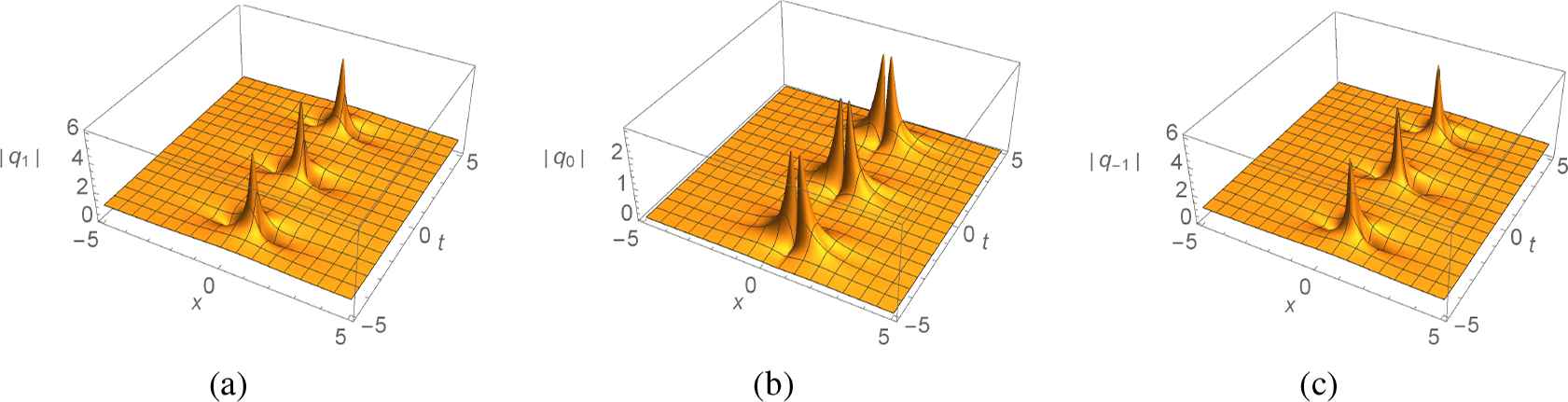
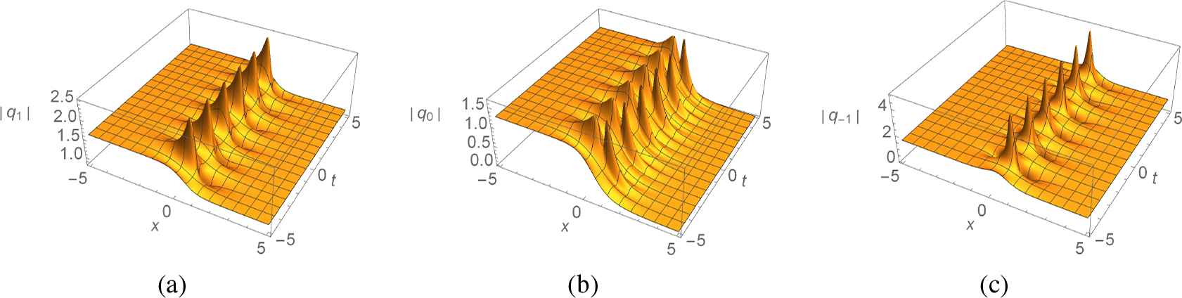
In case 3 it appears that the soliton solutions are regular only for full rank norming constants (detC1 ≠ 0), in analogy to what happens with zero boundary conditions [34]. In other words, no regular ferromagnetic solitons exist in case 3. Here we find dark solitons in the diagonal components of the potential and bright soliton solutions in the off-diagonal component. For a general discrete eigenvalue as in Fig. 2, we observe the spinor analog of Tajiri-Watanabe type solutions [4, 37]. For a pure imaginary discrete eigenvalue as in Fig. 3, we observe the analog of Kuznetsov-Ma breather solutions [4,23,26] that are periodic in t and homoclinic in x. For a discrete eigenvalue on the circle C0 as in Fig. 4, we observe solutions that behave like simple (non-oscillating) dark-bright solitons.

Fig. 2:

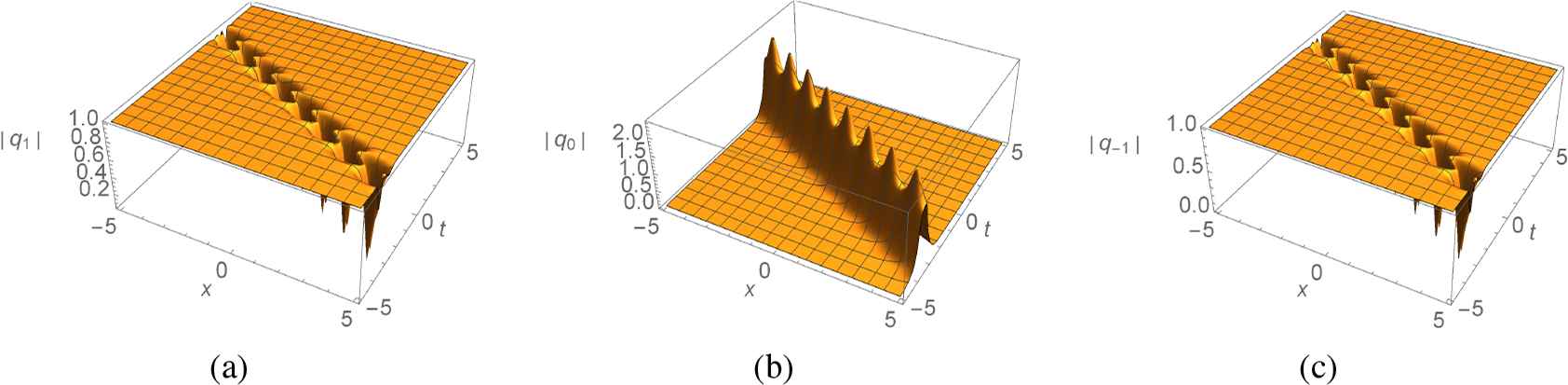
Case 3 (ν = 1), three components (q1, q0 and q−1 from left to right) with Q+ = I2, z1 = 1+2i, and norming constant entries c1 = 0, c0 = 1/2 + i, c−1 = 0 (detC1 ≠ 0)

Fig. 3:

Case 3 (ν = 1), three components (q1, q0 and q−1 from left to right) with Q+ = I2, z1 = 3i/2, and norming constant entries c1 = i, c0 = 2, c−1 = 3i/2 (detC1 ≠ 0)

Fig. 4:

Case 3 (ν = 1), three components (q1, q0 and q−1 from left to right) with Q+ = I2, z1=1/2+3i/2, and norming constant entries c1 = i, c0 = 2, c−1 = 3i/2 (detC1 ≠ 0)

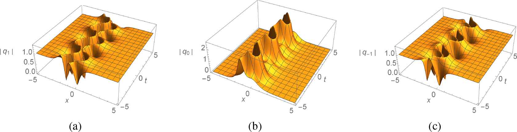
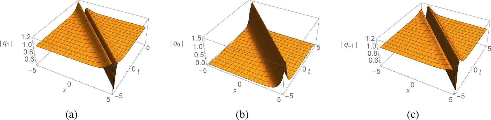
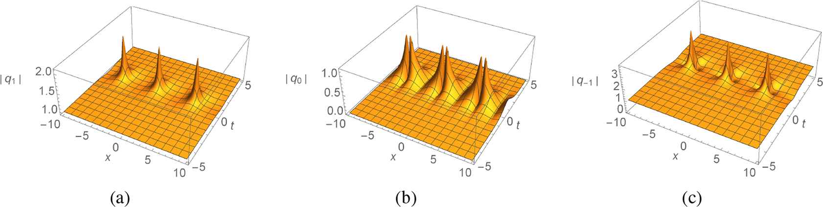
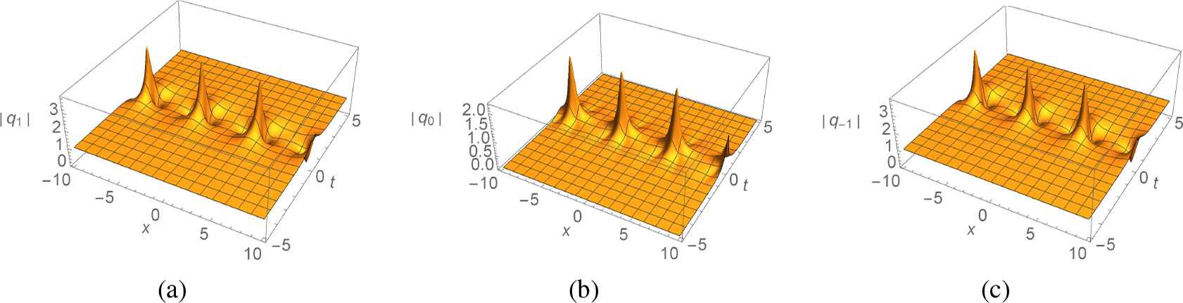
In case 4, we find regular soliton solutions both for norming constants C1 with detC1 = 0 and with detC1 ≠ 0. In general, when detC1 = 0, a shift in the norm of the background between Q and Q+ is observed, i.e., domain-wall type solutions appear; on the contrary, when detC1 ≠ 0, the background has the same asymptotic norm at +∞ and −∞. For a general discrete eigenvalue as in Fig. 5, we observe the analog of Tajiri-Watanabe type solutions. For a pure imaginary discrete eigenvalue as in Fig. 6 and Fig. 8, we observe the analog of Kuznetsov-Ma breather solutions that are periodic in t. For discrete eigenvalues on the circle C0 as in Fig. 7 and Fig. 9, we observe the analog of Akhmediev breather solutions [2, 4] that are periodic in x and homoclinic in t.

Fig. 5:

Case 4 (ν = −1), three components (q1, q0 and q−1 from left to right) with Q+ = I2, z1 = 1 + 2i, and norming constant entries c1 = 1, c0 = 2, c−1 = 4 (detC1 = 0)

Fig. 6:

Case 4 (ν = −1), three components (q1, q0 and q−1 from left to right) with Q+ = I2, z1 = 3i/2, and norming constant entries c1 = 3i/2, c0 = 1/2, c−1 = 2i (detC1 ≠ 0)

Fig. 8:

Case 4 (ν = −1), three components (q1, q0 and q−1 from left to right) with Q+ = I2, z1 = 2i, and norming constant entries c1 = 1, c0 = 2, c−1 = 4 (detC1 = 0)

Fig. 7:

Case 4 (ν = −1), three components (q1, q0 and q−1 from left to right) with Q+ = I2, z1=1/2+3i/2, and norming constant entries c1 = 1, c0 = 2, c−1 = 4 (detC1 = 0)

Fig. 9:

Case 4 (ν = −1), three components (q1, q0 and q−1 from left to right) with Q+ = I2, z1=1/2+3i/2, and norming constant entries c1 = 3i/2, c0 = 1/2, c−1 = 2i (detC1 ≠ 0)

5. Conclusion

In this work, we have developed the IST with nonzero boundary conditions for a class of matrix NLS equations whose reductions include the defocusing/focusing MNLS (cases 1 and 2), which have applications in three-component BECs, and two novel cases 3 and 4, which have applications in nonlinear optics and four-component fermionic condensates. We have provided a rigorous definition of norming constants that does not use unjustified analytic extensions of the scattering relations. We have properly accounted for all three symmetries in the potential matrix and the corresponding symmetries in the norming constants. The novel cases 3 and 4 present additional challenges in that, unlike cases 1 and 2, certain constraints are required on the norming constant in order to obtain regular soliton solutions. The large number of explicit solutions we have considered seem to suggest that the same constraints on the norming constants that guarantee regularity in the case of zero boundary conditions also work when nonzero boundary conditions are considered, but we plan to address this issue rigorously in a future work. The asymptotic analysis of the soliton solutions, and the soliton interactions are also deferred to future work.

Cases 3 and 4 are worth investigating in the context of multicolor optical spatiotemporal solitary waves created by interaction of light at a central frequency with two sideband waves both through cross-phase modulation and parametric four-wave mixing of opposite signs. On the other hand, the four-component spinor system could have applications in the recently discovered phenomenon of superconductivity in bilayer graphene [5].

Acknowledgments

AKO gratefully acknowledges support for this work from the UCCS graduate school under the Mentored Doctoral Fellowship grant. AKO and BP also thankfully acknowledge support from the National Science Foundation under grant DMS-1614601.

References

[6]F. Demontis, B. Prinari, C. van der Mee, and F. Vitale, The inverse scattering transform for the decofusing nonlinear Schrödinger equations with nonzero boundary conditions, Studies in Appl. Math, Vol. 131, 2013, pp. 1-40.
[8]L.D. Faddeev and L. A. Takhtajan, Hamiltonian Methods in the Theory of Solitons, Springer, Berlin, 1987.
[10]V.S. Gerdjikov, N.A. Kostov, and T.I. Valchev. BoseEinstein condensates with F = 1 and F = 2. Reductions and soliton interactions of multi-component NLS models in: “Proceedings of SPIE“ 7501, 75010W, S.M. Saltiel, A.A. Dreischuh, I.P. Christov (eds.), 2009
[23]E.A. Kuznetsov, Solitons in a parametrically unstable plasma, Sov. Phys. Dokl. (Engl. Tansl.), Vol. 22, 1977, pp. 507-508.
[26]Y.C. Ma, The perturbed plane-wave solutions of the cubic Schrödinger equation, Stud. in Appl. Math, Vol. 60, 1979, pp. 43-58.
[31]Y. Ohta, D.S. Wang, and J. Yang, General N-dark-dark solitons in the coupled nonlinear Schrödinger equations, Studies in Appl. Math, Vol. 127, 2011, pp. 345-371.
[34]B. Prinari, A. Ortiz, C. van der Mee, and M. Grabowski, Inverse scattering transform and solitons of square matrix nonlinear Schrödinger equations, Studies in Appl. Math, Vol. 141, 2018, pp. 308-352.
[35]Z. Qin and G. Mu, Matter rogue waves in an F = 1 spinor Bose-Einstein condensate, Phys. Rev. E, Vol. 86, 2012, pp. 036601.
[39]T. Tsuchida. Exact solutions of multicomponent nonlinear Schrödinger equations under general planewave boundary conditions, arXiv 1308.6623v2 (2013)
[44]X. Zhou, Direct and inverse scattering transforms with arbitrary spectral singularities, Commun. Pure Appl. Math, Vol. 42, 1989, pp. 895-938.
Journal
Journal of Nonlinear Mathematical Physics
Volume-Issue
27 - 1
Pages
130 - 161
Publication Date
2019/10/25
ISSN (Online)
1776-0852
ISSN (Print)
1402-9251
DOI
10.1080/14029251.2020.1683996How to use a DOI?
Copyright
© 2020 The Authors. Published by Atlantis and Taylor & Francis
Open Access
This is an open access article distributed under the CC BY-NC 4.0 license (http://creativecommons.org/licenses/by-nc/4.0/).

Cite this article

TY  - JOUR
AU  - Alyssa K. Ortiz
AU  - Barbara Prinari
PY  - 2019
DA  - 2019/10/25
TI  - Inverse Scattering Transform and Solitons for Square Matrix Nonlinear Schrödinger Equations with Mixed Sign Reductions and Nonzero Boundary Conditions
JO  - Journal of Nonlinear Mathematical Physics
SP  - 130
EP  - 161
VL  - 27
IS  - 1
SN  - 1776-0852
UR  - https://doi.org/10.1080/14029251.2020.1683996
DO  - 10.1080/14029251.2020.1683996
ID  - Ortiz2019
ER  -