
Understanding crude oil import demand behaviour in Africa: The Ghana case
- DOI
- 10.1016/j.joat.2017.11.002How to use a DOI?
- Keywords
- F10; Q11; Q31; Q41; Q48
- Abstract
As in many African countries, crude oil importation is a major drain on the economy of Ghana. We estimate short-run and long-run import demand models for crude oil using data over the period 1980–2012. Results show that demand for crude oil is price inelastic in the short-run but elastic in the long-run. Other important drivers of crude oil import are the real effective exchange rate, domestic oil production and population growth. Income is found to be the strongest driver of crude oil demand. Policy implications of our results are presented.
- Copyright
- © 2017 Afreximbank. Production and hosting by Elsevier B.V. All rights reserved.
- Open Access
- This is an open access article under the CC BY-NC license (http://creativecommons.org/licences/by-nc/4.0/).
1. Introduction
Crude oil is a major driver of businesses, manufacturing, transportation, as well as maritime trade at the national, regional and global levels. The pursuit of higher economic growth implies the need for adequate supply of crude oil and its constituent products such as gasoline, liquefied petroleum gas (LPG), and kerosene for the domestic, industrial, and agricultural and transport sectors of any economy. Since the episodes of the global oil price hikes in the 1970s and during the 2007–2008 crisis period where (light blend Brent) crude oil price shot up from US$25 per barrel in January 2000 to US$134 in July 2008 (International Monetary Fund, 2017), interest in the analysis of price and demand dynamics of crude oil has increased. Although crude prices have fallen substantially recently, they still represent large portions of African countries’ budgets (see International Monetary Fund, 2015; Essandoh-Yeddu and Yalamova, 2015; The Economist, 2016). Understanding the dynamics of the petroleum subsector and demand for petroleum and related products is therefore crucial for policy purposes.
Ghana achieved lower middle income status in 2006 after a rebasing of the national accounts. With a chequered economic history characterized by a series of fluctuating revenue inflows and losses from commodity exports (mainly gold, cocoa and timber), Ghana has since the last two decades posted considerable growth rates. Real gross domestic product (GDP) growth has hovered around 5% since 2003, hitting an all-time high of 15% in 2011. The rapid growth of the economy might imply increase demand for energy, especially crude oil. Ghana has traditionally been a net importer of crude oil, the price of which is determined on the international market. As a small and open economy, Ghana is often vulnerable to oil price shocks in the event of any significant price fluctuations. Total domestic oil consumption continues to rise while production has remained largely constant from 1980 until 2010 when commercial production came on-stream. Consequently, domestic production surged significantly from almost 9000 barrels a day in 2010 to about 80,000 barrels by 2012. From 16,000 barrels per day in 1980, crude oil consumption stood at 64,000 barrels per day in 2012 (see Figs. 1 and 2). In 2009 and 2010 alone, crude oil consumption grew by about 21.4% and 20.2%, respectively.
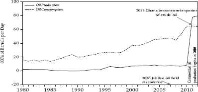
Ghana’s crude oil production and consumption (1980–2012).
Data source: International Energy Statistics, U.S. EIA database.
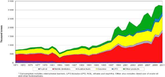
Consumption of oil products.
Source: IEA, 2013.
Crude oil constitutes a significant share of total imports and a major contributor to the worsening trade balance and overall balance of payment (BOP) position in Ghana (Table 1 and Fig. 3). Crude oil imports have increased from US$307 million in 1980 to US$3.2 billion in 2011 (about 11% annual average growth over the last 30 years). Daily crude oil imports for power generation for domestic and commercial uses amounts to US$30 m (World Bank, 2013). Another worrying trend fiscally is that Ghana continues to finance significant shares of the crude oil import bills from export earnings. For example, in 2007, about 50.2% of the country’s export earnings were used to finance crude oil purchases (Table 1). Meanwhile, Ghana’s crude oil imports are estimated to be in excess of US$3 billion per annum between 2012 and 2018 (Fig. 3).
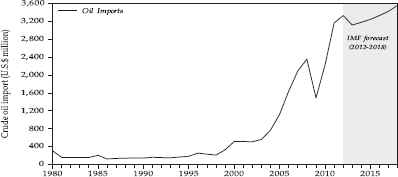
Trends in Ghana’s crude oil imports (US$ million).
Data source: World Economic Outlook, April 2013, IMF.
| 2000 | 2005 | 2006 | 2007 | 2008 | 2009 | 2010 | 2011** | 2012 | |
|---|---|---|---|---|---|---|---|---|---|
| Merchandise imports (f.o.b) | 2766.6 | 5347.3 | 6753.7 | 8066.1 | 10,268.5 | 8046.3 | 10,922.1 | 15,837.7 | 17,763.2 |
| Non-oil import | 2246.4 | 4217.9 | 5107.5 | 5971.1 | 7911.8 | 6557.3 | 8686.2 | 12,672.3 | 14,432.6 |
| Oil import | 520.1 | 1129.4 | 1646.2 | 2095.0 | 2356.7 | 1489.0 | 2235.9 | 3165.4 | 3330.2 |
| Oil import/non-oil import | 23.2 | 26.8 | 32.2 | 35.1 | 29.8 | 22.7 | 25.7 | 25.0 | 23.1 |
| Merchandise exports (f.o.b) | 1936.3 | 2802.2 | 3726.7 | 4172.1 | 5269.7 | 5839.7 | 7960.1 | 12,785.4 | 13,542.8 |
| Merchandise trade Balance* | 830.2 | 2545.1 | 3027.0 | 3894.0 | 4998.8 | 2206.6 | 2962.0 | 3052.3 | 4220.4 |
| Oil import/trade Balance (%) | 62.6 | 44.4 | 54.4 | 53.8 | 47.1 | 67.5 | 75.5 | 103.7 | 78.9 |
| Oil import/total import (%) | 18.8 | 21.1 | 24.4 | 26.0 | 23.0 | 18.5 | 20.5 | 20.0 | 18.7 |
| Oil import/total exports (%) | 26.9 | 40.3 | 44.2 | 50.2 | 44.7 | 25.5 | 28.1 | 24.8 | 24.6 |
| Nominal GDP($ million) | 4982.8 | 10,731.9 | 20,410.3 | 24,757.6 | 28,528.0 | 25,977.9 | 32,174.2 | 39,565.0 | 40,710.8 |
| Oil import/GDP (%) | 10.4 | 10.5 | 8.1 | 8.5 | 8.3 | 5.7 | 6.9 | 8.0 | 8.2 |
Notes: * Deficit trade balance;
Gas imports from Q1 added to oil imports; f.o.b denotes freight on board.
Trends in oil imports and related indicators, Ghana (in US$ million unless otherwise stated).
Sources: Bank of Ghana; WDI, World Bank.
With a view to influencing policy-making with regard to energy use and related matters, this paper empirically analyses the determinants of crude oil import based on data from Ghana. It is one of the few studies on African countries. Our paper is closest to Ziramba (2010), who estimated income and price elasticities of crude oil import demand in South Africa. Against this background, we utilize the autoregressive distributed lag model (ARDL) to empirically estimate both short-run and long-run price and income elasticities of oil import in Ghana. We also control for other potentially relevant drivers such as real effective exchange rate (REER), domestic crude oil production and population growth.
The rest of the paper is structured as follows: Section 2 briefly reviews related literature. Econometric methodology and data issues are discussed in Section 3, while a discussion of empirical results is presented in Section 4. The paper concludes in Section 5 with some policy implications.
2. Literature review
There is a plethora of empirical studies on energy demand in developed, emerging, and developing countries. Several of these have investigated the determinants of aggregate demand or disaggregated components of different energy types. Recent studies include Ghouri (2001), Krichene (2002), Cooper (2003), Alves and Bueno (2003), Dées et al. (2007) and Altinay (2007).1 The results are mixed. While several find inelastic demand with respect to both oil price and real income, others reveal price inelastic but income elastic oil demand. For example, Altinay (2007) estimated short-run and long-run elasticities of crude oil demand in Turkey using the ARDL method, with price and income coefficients of −0.104/0.635 and −0.182/0.608 in the short-run and long-run, respectively. In another study of 12 Middle Eastern countries, Narayan and Smyth (2007) finds that income elasticity differs across countries but consumers are insensitive to price changes, suggesting that demand for oil in the Middle East is driven primarily by income.
Zhao and Wu (2007) examined the factors that determined oil imports into China. They considered crude oil price, domestic energy production (including crude oil), industrial output and total traffic volume as potential determinants. They found a significantly positive and inelastic price demand for oil imports, with crude oil price playing a trivial role in China’s oil imports. The most important factors driving oil import demand in China are industrial output, local total energy output and the transport sector (total freight traffic and passenger traffic elasticities were 1.92 and 3.60, respectively). Another study on China by Xiong and Wu (2009) identified oil, GDP, population growth and share of the industrial sector in GDP as the drivers of crude oil demand. Similarly, Jabir (2009) finds that the US GDP plays a leading role together with domestic oil production in determining oil imports. Studies by Pedregal et al. (2009) and Sa’ad (2009) also find that the main driver of demand for crude oil products in Spain and Indonesia is real income rather than price. And, for some African evidence, Iwayemi et al. (2010) finds that petroleum products are both price and income inelastic in Nigeria. For greater details on the various studies, including methodologies, Table 2 summarizes (long-run) results of selected studies of crude oil/gasoline demand elasticities.
| Study | Country(ies) | Price elasticity | Income elasticity | Modelling technique | Study period |
|---|---|---|---|---|---|
| Ghouri (2001) | USA | −0.045 | 0.989 | Almon polynomial | 1980–1999 |
| Canada | −0.06 | 1.08 | distributed | ||
| Mexico | −0.05 | 0.84 | lag model | ||
| Krichene (2002) | World | −0.005 –0.13 | 0.6 1.80 | Simultaneous equation model (SEM) | 1918–1999 |
| Cooper (2003) | USA (+ 22 other countries) | −0.06 | 1.05 | Nerlove’s partial adjustment | 1979–2000 |
| Alves and Bueno (2003) | Brazil | −0.465 | 0.122 | Engle and Granger cointegration | 1974–1999 |
| Dées et al. (2007) | World | 0.17 0.98 | Quarterly macroeconometric model | 1984:1–2002:2 | |
| Altinay (2007) | Turkey | −0.18 | 0.61 | ARDL | 1980–2005 |
| Narayan and Smyth (2007) | Panel of 12 Middle East countries |
−0.015 | 1.014 | DOLS & FMOLS | 1971–2002 |
| Akinboade et al. (2008) | South Africa | −0.47 | 0.36 | ARDL | 1978–2005 |
| Ghosh (2009) | India | −0.63 | 1.97 | ARDL | 1970–2006 |
| Sa’ad (2009) | Indonesia | −0.15 −0.16 | 0.86 0.88 | ARDL | 1970–2005 |
| Pedregal et al. (2009) | Spain | −0.051 | 0.441 | Unobserved components model (UCM) | 1984:1–2006:12 |
| Broadstock and Hunt (2010) | UK | −0.12 | 0.57 | Structural time series model | 1960–2007 |
| Askari and Krichene (2010) | World | −0.002 | 0.020 | Simultaneous equation model (SEM) | 1970Q1–2008:Q4 |
| Ziramba (2010) | South Africa | −0.147 | 0.429 | Johansen cointegration analysis | 1980–2006 |
| Dargay and Gately (2010) | 30 OECDs | −0.60 | 0.80 | Reduced-form model with country fixed effects | 1971–2008 |
| Moore (2011) | Barbados | −0.552 | 0.91 | ARDL | 1998:1–2009:12 |
| Sentenac-Chemin (2012) | US | −0.28 | 0.60 | Cointegration technique | 1978–2005 |
Selected empirical long-run elasticities.
3. Methodology and data
3.1. Model specification and data
Following from the standard framework of modelling energy demand which is derived from the Marshallian demand theory for goods and services, we formulate our basic crude oil import demand model, consistent with the literature, as a function of real income and international price of crude oil. Incorporating other potential drivers, the real value of crude oil import is specified as a function of real GDP, real price of oil, real effective exchange rate (REER), domestic crude oil production (Oilprd) and rate of growth of population (POPG) as:
The model is formulated in logarithmic (ln) form except for the population variable which is in growth rate, so that the parameters represent elasticities, which are expected to assume the usual standard signs from demand theory: α1 < 0 and α2 > 0.
Among the control variables, POPG, measured by the annual population growth rate, is expected to have a positive coefficient. The inclusion of REER in the demand equation is important because oil price on the world market is quoted in US dollars, and changes in the exchange rate of the local currency against the US$ would affect the domestic price of oil and the real value of financial assets/ wealth and hence the demand for oil. The REER variable is defined such that an increase implies real appreciation of Ghana’s currency (GH¢) against the US$. Therefore, real appreciation of the local currency against the US$ should stimulate aggregate demand and hence a higher demand for crude oil. Also, domestic crude oil production could have a substitution effect for imported crude; hence we expect it to have a negative effect on crude oil demand.
We estimate the model using annual time series data for the period 1980–2012. Data used in this paper have been sourced from the International Financial Statistics (IFS), Fiscal Affairs Department database and World Economic Outlook of the IMF, the World Bank’s World Development Indicators (WDI), Ghana Statistical Service, and the Energy Information Administration (EIA) of the US Department of Energy (see Table 3 for summary statistics of data).
| Variables | Definition | Obs. | Mean | Std. Dev. | Min. | Max. |
|---|---|---|---|---|---|---|
| OilM | Annual crude oil import, US$ million | 33 | 729.7 | 921.3 | 127 | 3330 |
| OilPrd | Domestic oil production (1000 barrels per day) | 33 | 8.631 | 18.31 | 0.0900 | 79.63 |
| GDP | GDP in 2005 constant price, US$ million | 33 | 8169 | 3903 | 3816 | 18,374 |
| OilP | Average nominal world crude oil price (US$ per barrel) | 33 | 53.27 | 28.82 | 17.91 | 113.6 |
| REER | Real effective exchange rate index (2005 = 100) | 33 | 375.3 | 724.6 | 86.80 | 3579 |
| POPG | Annual population growth rate (%) | 33 | 2.658 | 0.332 | 2.175 | 3.482 |
Descriptive statistics.
3.2. Econometric estimation
In order to estimate short-run and long-run determinants of crude oil import demand, we use the ARDL modelling approach by Pesaran et al. (2001). This approach involves estimating a dynamic model by incorporating the lags of the dependent variable as well as the lagged and contemporaneous values of the independent variables. The short-run components are then estimated directly while the long-run effects are obtained indirectly. In this study, we utilize the bounds test for cointegration analysis within the ARDL framework. An advantage of the ARDL modelling approach over other cointegration procedures is that it has better finite sample properties, unlike the Engle and Granger two-step and Johansen maximum likelihood approaches which suffer from small sample bias. Hence the ARDL model is best suited for our estimation given our small sample. Furthermore, ARDL is relatively flexible, as it is applicable on I(1) or I(0) series and a combination of the two; hence pre-testing for the order of integration of the variables is generally not a pre-requisite. However, even though the ARDL framework does not require pre-testing of the variables for unit root, we need to ascertain the presence or otherwise of higher order integrated series such as I(2) which can invalidate the modelling process.
We implement the ARDL approach in two main steps. First, we test for cointegration to ascertain whether there is any long-run equilibrium relationship among the variables in the model to be estimated. If cointegration is established, we then estimate the long-run coefficients and the associated short-run parameters. The ARDL framework for Eq. (1) involves estimating the following restricted error correction model:
Cointegration among the variables is confirmed within the bounds test framework by testing the joint null hypothesis that the coefficients of the lagged level variables are significantly zero in Eq. (2). That is, if the null hypothesis represented by Ho : η1 = η2 = η3 = η4 = 0 is rejected, then the hypothesis of no cointegration is rejected against the alternative H1 : η1 ≠ 0, η2 ≠ 0, η3 ≠ 0, η4 ≠ 0 of cointegration using either a Wald or an F-test. We use the F-test in this paper. This is an F-test with a non-standard asymptotic distribution which is dependent on whether the included variables in the ARDL model are either I(0) or I(1), number of regressors, whether an intercept and/or a trend is included in the ARDL model, and the sample size (Pesaran et al., 2001; Ghosh, 2009). Pesaran et al. (2001) then provides two sets of critical values in testing for cointegration when the underlying variables are I(1) or I(0). If the calculated F-statistic exceeds the upper critical bound at conventional significance levels, then we can reject the null hypothesis of no cointegration. Conversely, if the calculated F-statistic falls below the lower critical bound, the null of no cointegration is not rejected. If it however falls within the band, then the test is inconclusive.
4. Results and discussion
4.1. Unit root results
The Phillips-Perron (PP)2 unit root procedure is used to test for non-stationarity of the underlying time series for the study. The PP procedure tests the null hypothesis of unit root against the alternative of stationarity of the series. Table 4 shows the results of the PP test. Including an intercept in the PP regression, the results show that all the variables contain unit root. Stationarity is however achieved after first differencing of the variables. Hence, we can conclude that all the variables are integrated of order one (i.e. I(1)), an indication of a possible long-run relationship among the variables.
| Variables | Level | First difference |
|---|---|---|
| lnOilM | 0.0734 | −6.6309*** |
| lnOilP | −0.9390 | −4.9609*** |
| lnGDP | 3.6440 | −3.0379** |
| lnREER | −1.3721 | −5.8032*** |
| lnOilPrd | −0.7136 | −5.2435*** |
| POPG | −1.7525 | −3.8722*** |
Notes: *** and ** denotes rejection of null hypothesis of unit root at the 1% and 5% levels, respectively. Test includes intercept. Critical values are based on MacKinnon (1996) one-sided p-values.
Phillips-Perron (PP) test.
4.2. Results of cointegration test
The results for the bounds test for cointegration relation are reported in Table 5. Tests for cointegration are made using four different specifications. The results show the existence of long-run equilibrium relationship in the case where oil import demand is modelled as a function of only oil price and real output. Here, the F-statistic of 6.07 exceeds the upper critical bounds at both the 5% and 10% levels. Thus, oil price and economic activity can be said to be long-run drivers of crude oil demand in model (1). The inclusion of additional variables also reveal significant cointegration relationship between crude oil demand and oil price, real GDP and a combination of either real effective exchange rate, domestic crude oil production and/ or population growth. Hence, we can conclude that international oil price, real output, a measure of Ghana’s international competitiveness (REER) and the rate of population growth are long-run drivers of real crude oil import demand in Ghana. We then proceed to estimate the long-run elasticities and the associated error-correction models in the next section.
| Dependent variable | F-statistics | Critical bounds | |||
|---|---|---|---|---|---|
| 5% | 10% | ||||
| I(1) | I(0) | I(1) | I(0) | ||
| FOilM(OilM|OilP,GDP) | 6.07** | 4.38 | 5.57 | 3.50 | 4.57 |
| 3.36 | 4.78 | 2.75 | 3.99 | ||
| FOilM(OilM|OilP,GDP,REER,POPG) | 8.14** | ||||
| FOilM(OilM|OilP,GDP,REER,OilPrd) | 7.49** | ||||
| FOilM(OilM|OilP,GDP,REER,OilPrd,POPG) | 6.18** | 3.09 | 4.54 | 2.57 | 3.82 |
Notes: ** denotes statistical significance at the 5% level.
Bounds test for cointegration.
4.3. Estimated long-run and short-run results
The results of the estimated long-run and short-run elasticities are reported in Table 6. The upper panel (A) contains the long-run estimates while the results for the corresponding short-run elasticities are shown in panel B. These results reflect adjusted price elasticities from the original estimates (see Table A1 in Appendix for the unadjusted oil price elasticities). The adjustment is necessary since import values, rather than volume, are used for the outcome variable (i.e. real crude oil import). If uncorrected, this is likely to result in inaccurate estimates of the price elasticity,3 hence the correction. The corresponding t-ratios for the short-run and long-run price elasticities have also been adjusted accordingly.4
| Variables/models | (1) | (2) | (3) | (4) |
|---|---|---|---|---|
| Panel A: long-run elasticities | Dependent variable: lnOilM | |||
| lnOilP | −1.277(−6.47)*** | −1.332(−8.10)*** | −1.161(−5.08)*** | −1.451(−7.18)*** |
| lnGDP | 1.638(5.36)*** | 2.055(7.93)*** | 1.970(3.78)*** | 2.632(6.15)*** |
| lnREER | 0.428(2.52)** | 0.490(1.86)* | 0.669(2.54)** | |
| lnOilPrd | −0.232(−1.82)* | −0.126(−1.45) | ||
| POPG | 0.143(0.28) | −1.819(−1.39) | ||
| Constant | −13.349(−4.80)*** | −19.684(−5.54)*** | −13.695(−1.70) | −25.342(−5.18)*** |
| Panel B: short-run elasticities | Dependent variable: Δ ln OilM | |||
| ΔlnOilP | −0.340 (2.48)** | −0.379 (3.18)*** | −0.209 (1.45) | −0.251 (2.26)** |
| ΔlnOilpt − 1 | −0.768 (5.93)*** | −0.765 (6.33)*** | −0.656 (5.49)*** | |
| ΔlnGDP | 0.524 (2.53)** | 0.996 (3.79)*** | 0.844 (2.54)** | −1.483 (−0.99) |
| ΔlnREER | −0.090 (−0.98) | −0.073 (−0.79) | −0.10335 (−0.88) | |
| ΔlnREERt − 1 | −0.364 (−4.29)*** | −0.353 (−4.36)*** | −0.333 (−4.35)*** | |
| ΔlnOilPrd | −0.099 (−2.12)** | −0.058 (−1.49) | ||
| ΔPOPG | 0.814 (2.02)* | −1.690 (−1.15) | ||
| ΔPOPGt − 1 | 2.076 (1.83)* | |||
| ECTt − 1 | −0.320 (−3.59)*** | −0.485 (−4.99)*** | −0.428 (−4.5773)*** | −0.465 (−5.67)*** |
| Regression statistics and diagnostic tests | ||||
| R2 | 0.730 | 0.852 | 0.879 | 0.861 |
| 0.681 | 0.774 | 0.798 | 0.788 | |
| F-Stat. | 19.8631[0.000] | 15.626[0.000] | 14.492[0.000] | 16.833[0.000] |
| DW-statistic | 1.98 | 2.46 | 2.55 | 2.27 |
| Serial correlation: χSC | 0.007[0.979] | 2.204[0.138] | 3.736[0.053] | 1.098[0.295] |
| Functional form: χFN | 0.481[0.488] | 3.888[0.049] | 3.777[0.052] | 2.883[0.090] |
| Normality: χN | 7.648[0.022] | 0.134[0.935] | 0.403[0.817] | 1.577[0.455] |
| Heteroscedasticity: χHET | 0.072[0.789] | 0.607[0.436] | 0.004[0.984] | 0.078[0.778] |
| CUSUM/CUSUMQ | Stable | Stable | Stable | Stable |
Notes: ***, ** and * denote statistical significance at the 1%, 5% and 10% levels, respectively. Optimal ARDL model selected based on the Schwarz Bayesian/Information Criterion (SIC). Values in parenthesis () and [] are t-statistics and p-values, respectively. The price adjusted coefficient is computed as (
Price-adjusted short-run and long-run elasticities.
Before proceeding to discuss the actual results, we first assess the appropriateness of the estimated short-run model. The estimated coefficients of the error correction terms (ECTt − 1) are correctly signed (negative) and statistically significant. This implies that following any shocks to the model, long-run equilibrium could be restored through an adjustment process. Specifically, a 1% shock to say model (3) implies an annual adjustment in long-run disequilibrium by 43%. That is, 43% of previous period disequilibrium can be corrected in the current period. Diagnostic tests applied to the residuals of the short-run model suggest the errors meet the usual i.i.d. requirements: no serial correlation, correct functional form, normality as well as constant variances. Lastly, stability tests on the parameters were assessed using Brown et al. (1975) cumulative sum of recursive residuals (CUSUM) and the cumulative sum of squares of residuals (CUSUMQ). In all the estimated models, both CUSUM and CUSUMQ tests indicate parameter stability given that the estimated statistics of each test fall within the 5% critical bounds.5
According to the results, import demand for crude oil in Ghana is price inelastic in the short-run but elastic in the long-run. Expectedly, Table 6 shows a highly significant inverse relationship between oil price and crude oil import demand in the long-run, suggested by models (1)–(4). A 10% hike in oil price on the international commodities market would be expected to depress import demand for crude oil in the range of between 11% and 14% in the long-run. Similarly, import demand for crude responds negatively to oil price in the short-run albeit inelastic in all estimated models (see Table 6, panel B). The results are significant for all current and one-period lagged estimates of international crude oil price, except for column (3) where the price effect is insignificant. The inelastic demand to oil price changes in the short-run could be due to lack of close substitutability for crude oil. The Ghanaian economy is heavily dependent on crude oil and related products for almost all productive economic activities ranging from electricity generation, transportation and manufacturing among others with almost close to no substitutes. Hence, it is quite plausible that price increases on the world market for crude would not necessarily lead to a very fast response in terms of demand cuts in Ghana, at least in the short-run. That is, the results imply that changes in oil prices do not have a big effect on crude oil demand in Ghana. The estimated coefficients of oil price in the short-run range between − 0.209 and −0.379 for current period price and −0.656 and −0.768 in the case of a one-period lag in oil price. In the long run, however, the quantity decreases in response to the higher oil price, apparently faster than the price increase, resulting in a much larger decrease in the import demanded.
Not surprisingly, though, we find that the strongest driver of high import demand for crude oil in Ghana is the level of income in both the long-run and short-run. All estimated coefficients of real income are positive and statistically significant at the 1% level. Thus demand for crude oil in Ghana is income elastic in the short- and long-run. The estimated elasticities of oil imports to income in the long-run imply that all things constant, an increase in real GDP by 1% would increase oil imports by between 1.6% and 2.6% in the long-run as given by estimates in columns (1)–(4). Thus, it is unsurprising that Ghana’s rapid economic growth in recent years has been associated with increasingly huge crude oil import bills.
The rather large magnitudes of the income estimates differ somewhat from those of other countries in the literature but compares well to a few. For example, Ghosh (2009) estimated long-run income elasticity of imported crude oil to be 1.97 for India. Similarly, Narayan and Smyth (2007) found an income elastic demand for oil in 7 out of the 12 Middle East countries considered in their study and an income elasticity of 1.014 for the entire panel.
Corroborating findings from Altinay (2007), Sa’ad (2009) and Ziramba (2010), however, we find short-run real income elasticity to be less than unity in the short-run. Specifically, our estimates are: 0.524, 0.996 and 0.844 in models (1)–(3), respectively. Albeit with a theoretically incorrect negative sign in model (4), the effect of real GDP on crude oil demand is statistically insignificant.
The role of the real effective exchange rate in the determination of real crude oil demand has received little attention in the literature. Apart from Askari and Krichene (2010) who explicitly included nominal effective exchange rate in their world crude oil demand model to account for monetary policy effects, we are not aware of any other studies on crude oil import demand that allow for exchange rate effects. However, since crude oil is priced in US dollars, the performance of the US dollar against international bilateral currencies would have an impact on the price of oil and hence demand for crude. For example, depreciation of the US dollar implies oil becomes relatively cheap in local currency terms for consumers in Ghana, for example, which could spur import demand for crude oil. Conversely, a real effective exchange rate depreciation of the US dollar would stimulate real economic activity and hence crude oil demand through its wealth effect arising from non-dollar denominated financial assets (Askari and Krichene, 2010). The preceding reasons could plausibly explain the effect of the REER variable in our real oil import demand models. For example, results in the long-run (columns 2, 3 and 4) show that real appreciation of the Ghanaian currency against the US dollar stimulates demand for crude oil with an inelastic effect. In contrast, it significantly reduces oil import demand in the short-run with a lag.
We further investigate whether domestic oil production could substitute for imported crude oil. Our estimates, in particular model (3), where all the other variables are accounted for, show that domestic oil production could potentially substitute for oil imports in both the short and long term. The magnitude of the estimated coefficient in the short-run of −0.099, however, indicates that the effect of increased oil production is almost negligible in the short term. An increase in domestic production of oil by say 10% would depress import demand for oil by only 0.9%, all things equal. In the long-run, however, the effect is much stronger, albeit still inelastic (−0.232). The inelastic effect of domestic oil production in the long-run suggests that domestic production in larger quantities would be required, given government policy, to significantly reduce dependency on foreign crude oil.
Finally, population growth could spur demand for crude oil. The effect of the annual growth rate in population is positive, as expected, but only marginally significant, in the short-run.
5. Conclusion and policy implications
This paper was motivated by the lack of in-depth empirical analysis of the drivers of crude oil import demand in the African context, particularly Ghana. It utilizes the autoregressive distribution lag model (ARDL) to estimate short-run and long-run demand determinants of crude oil import in Ghana. Annual data covering roughly three decades (1980–2012) was used for the empirical analysis.
The results of the paper are summarized as follows. First, we find evidence in support of cointegration (i.e. long-run equilibrium relationship) among the variables considered. Second, the results show that demand for imported crude oil is price inelastic in the short-run but elastic in the long-run. Our results contrast with those of earlier studies on South Africa and Nigeria where price was inelastic in the long-run, but compare quite well with their short-run results (see Ziramba, 2010; Adewuyi, 2016).6
Further, demand for crude oil was found to be income inelastic in the short-run but elastic in the long-run. The coefficient of income is theoretically consistent (i.e. positive) and corroborates earlier African case studies (e.g. Akinboade et al., 2008; Ziramba, 2010; Adewuyi, 2016). The results also show the significant role of real effective exchange rate in driving crude oil import decisions in Ghana in the short- and long-term. While the effect of this variable is positive and significant in the long-run, however, we find only the one-period lag effect to be significant in the short-run and inelastic in each case. Another important finding relates to the effect of domestic oil production and population growth on imports. Domestic oil production holds some promise in substituting for heavy dependence on imported crude, while population growth induces only a marginally significant increase in import demand, at least in the short-run.
The foregoing results have some important policy implications. That crude oil imports are price-elastic in the long run suggests that allowing the domestic price to reflect the international crude price might be an effective policy to help curb oil imports. Another demand-side suggestion would be that authorities should increase and sustain investment/switching into cleaner alternative energy sources such as natural gas, biofuel and solar, among others, for a more sustainable energy generation in the future. Such a strategy might be required especially given our finding of an inelastic responsiveness of oil imports to domestic production. The current natural gas production facility due to process gas from the Jubilee and TEN oil fields is an important strategic asset that government and investors could take advantage of in order to meet the country’s energy needs. This would require efficient utilization and management of the physical infrastructure and financial resources of this national asset which could potentially facilitate Ghana’s future energy security. This, if efficiently done and sustained, may reduce Ghana’s high dependence on the unreliable supply of crude oil from the West African Gas Pipelines in the medium-to-long-term.
Additionally, we find that exchange rate policies in Ghana may have contrasting effects on crude oil imports. While exchange rate policy dynamics might have a dampening effect on oil demand in the short-run, the opposite effect may occur in the long-term. Thus fiscal and monetary authorities should be mindful of these potential opposing effects in the implementation of exchange rate policies.
Population growth, which is an indication of an expanding local market size, appears to be an important driver of crude oil import demand in Ghana. The implication is that the oil import bill is likely to continue surging in the face of expanding energy demand via positive population growth (rural and urban). Thus analysis of crude oil demand projections in demand management by authorities needs to carefully consider this variable in their decisions.
Finally, it may seem reasonable for government to reconsider its decision to continue to lift and export almost all crude oil extracted from Ghana’s oil fields. This may appear a plausible policy shift given that domestic crude oil production is significant in substituting for imported crude. A deliberate policy stance by government to gradually source significant crude oil requirements from its own oil fields would likely reduce the increasing import bill substantially and hence the persistent trade and fiscal deficits. It may also reduce the effects of price and exchange rate volatility on the economy and boost growth in the long-term.
Acknowledgements
The author acknowledges with appreciation comments and helpful editorial assistance from the Editor-in-Chief of the journal, Professor Augustin Fosu, on previous versions of this paper. I am also grateful for additional helpful comments from an anonymous referee which helped in improving the paper. Constructive feedback from seminar participants at the Department of Economics, Swedish University of Agricultural Sciences (SLU) in October 2013 are duly acknowledged. Finally, I thank George Adu (KNUST) and Justice Tei Mensah (SLU) for providing useful feedback from their review of initial versions of the manuscript. Any remaining errors are, however, mine.
Appendix A
| Variables/models | (1) | (2) | (3) | (4) |
|---|---|---|---|---|
| Panel A: long-run elasticities | Dependent variable: ln OilM | |||
| lnOilP | −0.277(−1.40) | −0.332(−2.02)* | −0.161(−0.70) | −0.451(−2.23)** |
| lnGDP | 1.638(5.36)*** | 2.055(7.93)*** | 1.970(3.78)*** | 2.632(6.15)*** |
| lnREER | 0.428(2.52)** | 0.490(1.86)* | 0.669(2.54)** | |
| lnOilPrd | −0.232(−1.82)* | −0.126(−1.45) | ||
| POPG | 0.143(0.28) | −1.819(−1.39) | ||
| Constant | −13.349(−4.80)*** | −19.684(−5.54)*** | −13.695(−1.70) | −25.342(−5.18)*** |
| Panel B: short-run elasticities | Dependent variable: Δ ln OilM | |||
| ΔlnOilP | 0.660 (4.82)*** | 0.621 (5.21)*** | 0.791 (5.50)*** | 0.749 (6.74)*** |
| ΔlnOilpt − 1 | 0.232 (1.79)* | 0.235 (1.94)* | 0.344 (2.88)*** | |
| ΔlnGDP | 0.524 (2.53)** | 0.996 (3.79)*** | 0.844 (2.54)** | −1.483 (−0.99) |
| ΔlnREER | −0.090 (−0.98) | −0.073 (−0.79) | −0.10335 (−0.88) | |
| ΔlnREERt − 1 | −0.364 (−4.29)*** | −0.353 (−4.36)*** | −0.333 (−4.35)*** | |
| ΔlnOilPrd | −0.099 (−2.12)** | −0.058 (−1.49) | ||
| ΔPOPG | 0.814 (2.02)* | −1.690 (−1.15) | ||
| ΔPOPGt − 1 | 2.076 (1.83)* | |||
| ECTt − 1 | −0.320 (−3.59)*** | −0.485 (−4.99)*** | −0.428 (−4.5773)*** | −0.465 (−5.67)*** |
| Regression statistics and diagnostic tests | ||||
| R2 | 0.730 | 0.852 | 0.879 | 0.861 |
| 0.681 | 0.774 | 0.798 | 0.788 | |
| F-Stat. | 19.8631[0.000] | 15.626[0.000] | 14.492[0.000] | 16.833[0.000] |
| DW-statistic | 1.98 | 2.46 | 2.55 | 2.27 |
| Serial correlation: χSC | 0.007[0.979] | 2.204[0.138] | 3.736[0.053] | 1.098[0.295] |
| Functional form: χFN | 0.481[0.488] | 3.888[0.049] | 3.777[0.052] | 2.883[0.090] |
| Normality: χN | 7.648[0.022] | 0.134[0.935] | 0.403[0.817] | 1.577[0.455] |
| Heteroscedasticity: χHET | 0.072[0.789] | 0.607[0.436] | 0.004[0.984] | 0.078[0.778] |
| CUSUM/CUSUMQ | Stable | Stable | Stable | Stable |
Notes: ***, ** and * denote statistical significance at the 1%, 5% and 10% levels, respectively. Optimal ARDL model selected based on the Schwarz Bayesian/Information Criterion (SIC). Values in parenthesis () and [] are t-statistics and p-values, respectively.
Unadjusted short-run and long-run elasticities.
Footnotes
Others include Narayan and Smyth (2007), Akinboade et al. (2008), Ghosh (2009), Sa’ad (2009), Pedregal et al. (2009), Broadstock and Hunt (2010), Askari and Krichene (2010), Ziramba (2010), Dargay and Gately (2010), Moore (2011), Ediger and Berk (2011), Sentenac-Chemin (2012).
The Phillips and Perron (1988) test is an alternative (nonparametric) method of controlling for serial correlation when testing for a unit root.
This situation might likely explain why the uncorrected short-run price elastic estimates are perversely positive (see Table A1 in the Appendix). We are grateful to the editor for making this observation and recommending the adjustment.
The t-ratio is computed as
CUSUM and CUSUMQ plots for each model are not shown but available from author on request.
The difference in the long-run estimate might be due to the adjustment we made in the initial estimates to reflect the fact that the usual dependent variable is the value, rather than volume, of imports.
References
Cite this article
TY  - JOUR
AU  - George Marbuah
PY  - 2018
DA  - 2018/02/13
TI  - Understanding crude oil import demand behaviour in Africa: The Ghana case
JO  - Journal of African Trade
SP  - 75
EP  - 87
VL  - 4
IS  - 1-2
SN  - 2214-8523
UR  - https://doi.org/10.1016/j.joat.2017.11.002
DO  - 10.1016/j.joat.2017.11.002
ID  - Marbuah2018
ER  -