
CHEAP: An Efficient Localized Area Coverage Maintenance Protocol for Wireless Sensor Networks
- DOI
- 10.2991/ijndc.k.201218.001How to use a DOI?
- Keywords
- Coverage hole; detection; recovery; location-allocation; tabu search; wireless sensor network
- Abstract
Over the course of operation, a wireless sensor network can experience failures that are detrimental to the underlying application’s objectives. In this paper, we address the problem of restoring coverage ratio of a damaged area (hole) using only the neighboring nodes. Most existing solutions fail to simultaneously prevent new holes formation, collisions, oscillations, cascaded movements, and overlapped areas. To do this, we propose an intersection points-based strategy to properly locate and characterize any type of coverage hole. Then, we allow nodes, whether or not redundant, to coordinate their movements and ranges in order to effectively eliminate the detected hole. We suggest for that purpose, a tabu search based optimization scheme along with a location-allocation model through a mixed integer linear program. Simulation results show that our protocol significantly increases the network’s resilience.
- Copyright
- © 2021 The Authors. Published by Atlantis Press B.V.
- Open Access
- This is an open access article distributed under the CC BY-NC 4.0 license (http://creativecommons.org/licenses/by-nc/4.0/).
1. INTRODUCTION
Wireless Sensor Networks (WSNs) are composed of a large number of tiny devices that are able to measure various physical quantities in their immediate environment. During the last two decades, WSNs have been utilized in many event-monitoring applications that are related to domains such as security, ecology, agriculture, transportation, or industry [1–3]. Unfortunately besides their limited capabilities, sensor nodes are inherently prone to failures [4], especially when they are randomly deployed in hostile environments. These failures can lead to the occurrence of uncovered areas also called holes that can be detrimental to network effectiveness [5]. Hence, coverage maintenance is of paramount importance to have any hope of prolonging network lifetime [6]. This process comprises two phases namely, detection and elimination.
When the underlying application requires a complete area coverage, hole detection use techniques originating from geometry, algebraic topology and graph theory [7–13]; whereas hole elimination solutions can exploit nodes’ redundancy, mobility or motility [8,14–18]. Detection strategies must be fast and accurate whereas recovery schemes must eliminate the best the coverage hole while minimizing energy consumption and overlapped areas. This process must avoid creating new holes and be applied to both closed and open holes. It is also desirable that the coverage recovery strategy is localized and considers scenarios involving nodes with different ranges. To address all these requirements some authors opt for hybrid solutions which are essentially based on both nodes’ sensing range adjustment (motility) and controlled movements (mobility) [19]. However, schemes commonly proposed usually struggle to simultaneously prevent undesirable effects such as new hole formation, collisions, and oscillations especially when nodes movements are constrained by obstacles.
In this paper, we propose to seamlessly combine mobility, redundancy control, and motility based strategies in order to further increase the network’s resilience. The main contributions of this work are as follows:
- •
a localized intersection points based coverage hole detection scheme that helps to discover in linear time any type of hole (closed, semi-open, open), to minimize the use of geographical information, and to reduce message overhead;
- •
a location-allocation [20,21] based model and a mixed integer linear programming formulation for the area coverage recovery problem. A fully distributed tabu-search based scheme is applied to make hole elimination decisions. Unlike most existing solutions, our strategy guarantees energy-efficiency and high coverage ratio by simultaneously preventing new holes formation, cascaded movements, collisions, oscillations, especially in the presence of obstacles;
- •
a novel metric (the coverage resilience index) to help better estimate coverage hole elimination protocols’ actual fault tolerance ability;
- •
extensive simulations using various scenarios are performed to validate the proposed algorithms. Results show that our scheme outperforms several recently proposed solutions with respect to the number displaced nodes, coverage ratio, total distance travelled, and energy consumption.
The rest of the paper is organized as follows: Section 2 surveys recent and significant related contributions; then, the proposed solution is detailed in Section 3; the performance evaluation process, the results, and discussions are presented in Section 4 followed by conclusion in Section 5.
2. RELATED WORK
Area coverage maintenance is a two-phase process encompassing hole detection and its elimination. Hole detection phase is aimed at providing maximum information (position, surface, shape, perimeter...) about the damaged areas (holes) resulting from a topology change. Once identified, holes must be healed using the least amount of resources.
2.1. Hole Detection
Area coverage hole detection is part of network boundary detection problem [22]. Methods commonly used for that purpose can be categorized into geometric, algebraic topology, graph theory, and analytic methods [23]. Accuracy and precision are the most important challenges to face, irrespective of the type of holes (close, open, semi-open). Techniques commonly used (virtual grid, intersection points, perimeter coverage, Voronoi tessellation, Delaunay triangulation...) mainly originate from computational geometry. They generally require nodes to know their exact positions. An et al. [24] proposed a combination of cells and triangles in order to reduce the computational complexity. However, this scheme is only limited to closed holes and homogeneous networks. Trong et al. [7] proposed a solution for dynamic holes. Besides detecting holes, this strategy is aimed at predicting the enlargement of their boundaries but has the drawback of increasing message overhead. Amgoth and Jana [8] suggest also using classical square grids. However, this strategy targets only closed holes.
Kang et al. [25] suggest a coordinate-free strategy based on the concept of critical boundary points i.e. intersection points which are not covered by any other node. Regrettably, finding such points is time consuming. Sahoo et al. [9] use a similar strategy except that it requires nodes to know their exact positions.
Huang and Tseng [26] used a perimeter coverage based strategy that regrettably requires also sensors to know their exact locations. In order to cope with this shortcoming, Bejenaro [27] suggests a concept called cyclic segment sequence which involves using nodes’ local polar coordinates. A hole is detected if every selected arc (segment) does not overlap with exactly two other segments. However, this method has a high computational complexity
Qui et al. [28] proposed a k-coverage Delaunay triangulation oriented strategy. Any hole is now detected if a voronoi cell is covered by less than k nodes. Although innovative, this method has a
Senouci et al. [30] suggest using a collaborative scheme triggered by duly identified stuck nodes. Hole discovery process is based on the classical message forwarding TENT rule [31]. However, this strategy is dedicated to only closed holes. Chu and Ssu [32] used a location-free strategy that explicitly considers obstacles. However, this scheme requires each node to previously collect three-hops neighborhood information. In order to quickly detect holes, Patra and Sau [12] proposed to find a base cycle i.e. a cycle in the subgraph induced by each node’s neighborhood. Regrettably, this technique is devoted to only closed holes.
To avoid using nodes exact locations, many authors suggest using techniques inspired by homotopy or homology to infer a simplicial complex from the network topology. However, Yan et al. [33] showed that it is impossible to detect with a Rips complex, certain types of holes including triangular holes, i.e. damaged areas enclosed by three nodes (two-simplexes). In a recent study, Šorbel et al. [11] used a spanning tree-based strategy for homological coverage verification. Small network segments are gradually merged into larger ones, until a Rips complex is obtained. This merging strategy is helpful to locally compute the first Betti number but hardly scalable since the spanning tree construction scheme is centralized.
2.2. Hole Elimination
Area coverage recovery is also a well studied topic in the literature. Solutions commonly proposed can be classified into redundancy, motility, and mobility based approaches.
Diongue and Thiare [34] proposed to maintain active some nodes (sentinels) so that they watch over their sleeping neighbors. This strategy combines node-based and link-based adaptation schemes. The link adaptation technique helps a sentinel to dynamically adjust its communication range according to link quality. On the other hand, node adaptation process consists of waking up redundant nodes to replace the failed sentinels. Unfortunately, this strategy fails to cope with large scale damages. Sharma and Sharma [18] propose a similar scheme to minimize movements by grouping nodes according to their overlapping coverage ratio. Each cluster is controlled by a node referred to as the Zone Monitor (ZM). When a cluster member fails, the ZM orders the sleeping redundant ones to be active in order to eliminate the resulting hole. Nodes’ mobility is only used if no redundant node is found. Despite a low message overhead, no solution is proposed to cope with ZM failures.
As for mobility-based solutions, they mainly rely on nodes’ locomotion abilities to replace failed neighbors especially after a large scale disaster. The challenges to face include the minimization of the number of candidates, overlapped areas, cascaded movements, the average distance travelled while avoiding collisions, oscillations and new holes formation. Strategies commonly found, involve using (attractive or repulsive) virtual forces inspired from quantum physics [35–37]. Li et al. [15] investigated using Tchebychev point instead of targeting traditional points such as centroid or Voronoi vertex. Nodes must seek such a point in their k-order Voronoi cell. This scheme is very useful in 3D environments and helps to minimize oscillations but does not consider obstacles. Habibi et al. [38] use geometric optimization formulation. Although, this strategy provides a high coverage ratio, it cannot prevent the formation of new holes. To cope with this shortcoming, Sahoo and Liao [39] suggest to replace nodes according to their degrees while limiting their movements. They proposed a nonlinear programming formulation combined to a triangulation based scheme. The latter is aimed at minimizing energy consumption due to mobility and coverage overlapping. Regrettably, candidates selection scheme does not consider nodes’ residual energy. Qiu and Shen [40] proposed a coordinate-free scheme that first constructs Delaunay triangles (i.e. triangles that have no other node inside) and then conducts nodes movements to meet conditions that suffice to ensure each triangle full coverage. New holes creation are avoided by ensuring that each node finds a safe area capable of preserving its coverage. However, this technique considers only closed holes and requires nodes to synchronize their movements. Saha and Das [16] addressed this problem for heterogeneous networks, but the proposed scheme cannot be applied to open holes. Khelil and Beghdad [41] proposed a self-deployment scheme to move nodes periodically toward the centroid of the polygon induced by the hole. However, such a strategy also requires nodes’ movements to be synchronized. Rout and Roy [42] apply a strategy that use obstacles and deployment boundaries as sources of repulsive forces exerting on nodes. This solution enhances coverage ratio and minimizes distance travelled but cannot prevent the formation of new holes. Zhao et al. [43] proposed a novel paradigm referred to as fruit fly optimization. The deployment zone is discretized with a virtual grid. All the uncovered areas exert on nodes (fruit flies), smells that are able to attract them to suitable areas. This strategy considers the presence of obstacles and quickly converges but can only be applied to homogeneous and dense networks. Ray and De [44] suggest instead, a glowworm based heuristic that minimizes the number of overlapped areas but fails to prevent new holes formation.
Solutions aiming at controlling specifically nodes’ sensing ranges are more recent [45,46]. Qu and Georgakopoulos [47] used a Voronoi diagram based scheme that allows each node to adjust its range in order to entirely cover its Voronoi cell and check its redundancy. However, this solution is dedicated to only closed holes. Amgoth and Jana [8] proposed a virtual grid based scheme where after neighbor discovery, each node must identify cells that it can cover respectively with its current range and maximum range. These information help nodes to find cells that are not covered by any neighbor and eventually detect holes. In that case, a detection message is sent to alert these neighbors. If such a message is not acknowledged, node must increase its range in order to cover those empty cells. Although precise, this strategy is memory and energy expensive since large messages are required.
So far, only a few solutions have considered hybrid strategies to eliminate area coverage holes. Guvesan and Yavuz [19] proposed to combine motility and mobility based approaches. Regrettably, this protocol applies only to networks composed of nodes equipped with directional antennas. Abolhasan et al. [48] suggest a potential game theory based strategy that allows nodes to move or adjust their sensing ranges more efficiently. However, this solution is devoted to only closed holes and does not prevent the formation of new holes. Joshita et al. [49] proposed to vary nodes’ sensing ranges along with a random mobility. This scheme helps to minimize the number of candidates and the number of overlapped areas, but also cannot prevent new holes to appear. Khedr et al. [50] suggest to only move redundant nodes and to add a pro-active scheme where nodes with low residual energy must alert neighbors in order to prevent hole formation. However, this strategy leads to collisions since some neighbors can move to the position of the alert’s sender before its actual death.
3. PROPOSED SOLUTION
In this section we first discuss the motivations and objectives of this paper. Then we describe the key assumptions before detailing our solution.
3.1. Motivations and Objectives
Most existing solutions essentially aim to detect and eliminate only closed holes. It is useful to design a solution that can efficiently deal with the main three types of holes (closed, semi-open, and open) regardless of the failure scale.
Few hybrid hole elimination schemes, have been proposed in the literature. They often combine sensing range adjustment (motility) or redundancy control to mobility strategies in order to further reduce nodes’ energy consumption. However, they fail to simultaneously face challenges such as overlapped areas, new holes formation, collisions, oscillations, and cascaded movements. This shortcoming need to be addressed especially in the presence of obstacles.
Furthermore, in most studies the performance evaluation process is commonly based on metrics which alone are not sufficient to actually capture the protocol’s resilience ability. Hence, a more precise metric should be proposed to better estimate network’s fault tolerance.
This paper is specifically aimed at minimizing:
- •
coverage hole detection and elimination time;
- •
travel distance, overlapped areas, number of candidates, and movements required to eliminate a hole regardless its type and location;
- •
risk of new holes formation especially at the network’s boundaries.
3.2. Assumptions
We make the following assumptions:
- •
nodes respectively use the classical Unit Disk Graph and Boolean disk coverage models to communicate and sense events;
- •
each node u’s communication and sensing ranges, respectively denoted by rc(u) and rs(u), are such that rc(u) ≥ 2 × rs(u);
- •
each node u knows its position coordinates (xu, yu) in the deployment zone A using the underlying localization protocol;
- •
each node u can estimate the transmission delay τ(u, v) and the round trip time rtt(u) with each neighbor v;
- •
two nodes u and v are neighbors (with two intersection points) if d(u, v) < (rs(u) + rs(v)) and d(u, v) > (rs(u) − rs(v)). d(u, v) denotes the euclidean distance between u and v. (rs(u) + rs(v)) − d(u, v) > = λ; where λ is a parameter set by the underlying application.
- •
nodes are capable of adjusting their communication and sensing ranges (motility);
- •
nodes are able to control their mobility;
- •
the process is supposed to take place in a two-dimensional euclidian space.
3.3. Description
In this section, we detail our solution referred to as Coverage Hole Elimination Adaptive Protocol (CHEAP). This localized message passing protocol consists of three phases namely: hole detection, hole characterization, and hole elimination (coverage recovery).
We need first to give some definitions that can help to gain a better understanding of our strategy.
Definition 1
(Coverage of a node) Let i be a point of the deployment zone denoted by A, the coverage of node u denoted by C(u) is such as C(u) = {i ∈ A: d(u, i) ≤ rs(u)}; where d(u, i) is the euclidean distance between i and u while rs(u) denotes the sensing range of node u.
Definition 2
(Perimeter of a node) Let i be a point in C(u) the coverage of node u while the perimeter of u denoted by P(u) such as P(u) = {i ∈ C(u): d(u, i) = rs(u)}.
Definition 3
(Parents of an intersection point) the parents (father and mother) of a point are the nodes of which sensing disks intersection has created this point. Formally, let i be a point of the deployment zone denoted by A. Let u and v two nodes, (u, v ∈ χ(i)) ⇔ (i ∈ P(u)) ^ (i ∈ P(v)). Where χ(i), P(u), and P(v) respectively denote the set of point i’s parents, the perimeter of u, and the perimeter of v.
Definition 4
(Uncovered arc of a node) Let P(u) be the perimeter of node u and N(u) the set of its neighbors. A part of P(u) denoted by
In order to simplify notations and discussions, each uncovered arc
Definition 5
(Adjacent uncovered arcs) Let i, j, k, and l be four points whose coordinates are respectively denoted by (xi, yi),(xj, yj), (xk, yk) and (xl, yl). The uncovered arcs
Definition 6
(Maneuver of a node) A maneuver is an action (displacement or range change) that a node u can perform in order to be usefully involved in a hole elimination process. Formally, a maneuver m is a vector such as m = (xo, yo, xd, yd, ro, rd) and
(xo, yo, xd, yd, ro, rd) respectively denote the current position’s abscissa, the current position’s ordinate, the destination’s abscissa, the destination’s ordinate, the current range, and the destination’s range of node u. Therefore:
if (xo ≠ xd) ∨ (yo ≠ yd), maneuver m implies node u’s displacement (mobility);
if (ro ≠ rd), maneuver m implies node u’s range change (motility).
Definition 7
(Elbow room of a node) node u’s elbow room denoted by Φ(u) is the set of its maneuvers. Formally, let xu and yu respectively denote the abscissa and the ordinate of node u. Let I be a set of maneuvers, and F(u) a family such as F(u) = {η(u): η(u) ⊆ N(u)}
η(u) is referred to as node u’s immobilized neighborhood.
Definition 8
(Redundant node) A node u is redundant if each point within its range is also covered by at least one of its immobilized neighbors. Formally, u is redundant iff
Definition 9
(Maximum Redundancy Zone) The Maximum Redundancy Zone (MRZ) of node u is the region delimited by the convex hull deriving from the cloud of the intersection points between neighbors that belong to node u’s immobilized neighborhood. Points located on this hull will be referred to as the Border Points; whereas the others will be referred to as the Interior Points. Let IP(u), IN(u) and MRZ(u) respectively denote the set of intersection points between node u and its neighbors, the set of intersection points between node u’s neighbors, and the set of border points on the convex hull of node u’s MRZ; formally,
Definition 10
(Incompatible maneuvers) Two maneuvers m = (xo, yo, xd, yd, ro, rd) and
- •
- •
- •
maneuvers m and
- •
maneuvers m and
Definition 11
(State of a node) Node u can enter into the following states:
Sleep (SLP),
Active (ACT),
Tentative (TNT),
Alert (ALRT),
Initiator (INIT),
Coordinator (CRD),
Candidate (CAND),
Move (MOV),
3.3.1. Hole detection phase
Each active node must periodically (re)discover its neighbors and check for the presence of a potential coverage hole, following this process:
- •
step 1: get all Type 1 intersection points (i.e. intersection points with each neighbor);
- •
step 2: get Type 2 intersection points (i.e. intersection points between neighbors);
- •
step 3: create a cloud from the two types of intersection points;
- •
step 4: construct a convex hull from the point cloud created;
- •
step 5: get from that hull the set of border points (i.e. points that are covered only by their parents); the latter set is referred to as the convex hull of the MRZ;
- •
step 6: check if the MRZ’s convex hull contains Type 1 intersections points; if so, a coverage hole exists; stop.
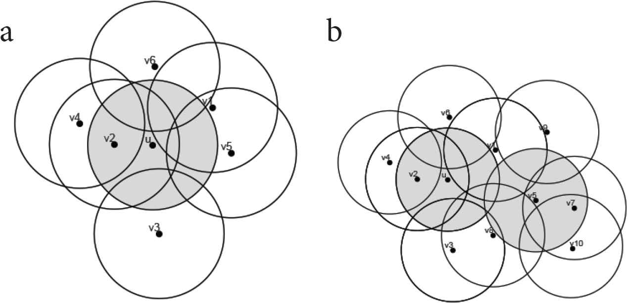
Let us see two examples. In Figure 1a node u constructs a convex hull (in red) from the cloud of intersection points, i.e. the intersection points with each neighbor (in white) and the ones between neighbors (in gray). Node u tries to derive from this first convex hull the one of the MRZ. To do this, node u focuses on points that are covered only by their parents, namely points bp1, bp2, bp3, and bp4, respectively covered by parents {v3, v4}, {v2, v4}, {v1, v2}, and {v2, v3}. There is no white point among them, therefore, there is no coverage hole. Note that, in this example the first convex hull and the one of the MRZ coincide; this is not always the case. Figure 1b shows another example where node u constructs a convex hull from a cloud of intersection points (white and gray). Then node u derives its MRZ’s convex hull composed of bp1, bp2, bp3, and bp4. However, two of these points (bp1 and bp2) are white. Node u concludes that arc
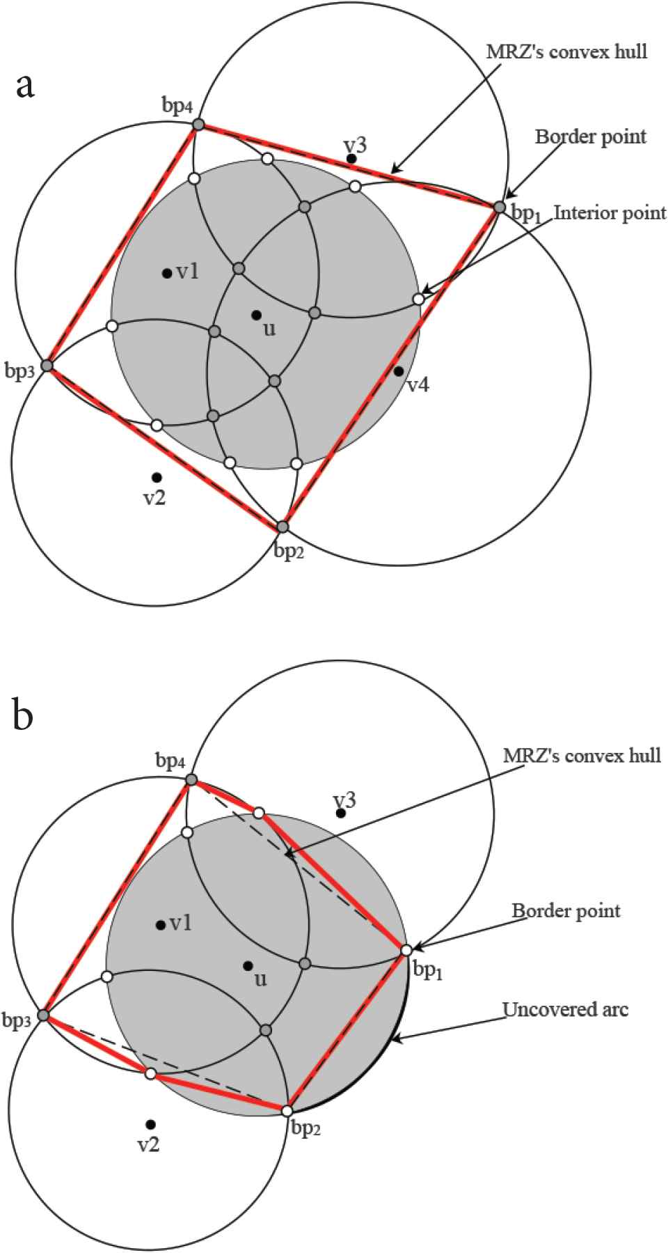
Construction of the Maximum Redundancy Zone (MRZ)’s convex hull (dotted) in order to detect a coverage hole by node u: (a) no coverage hole, no intersection point with neighbors found on this hull (b) coverage hole, two intersection points with neighbors found on this hull.
Note that, each node must store the parents’ identifiers (fi, mi) of all the intersection points i located on the convex hull of its MRZ. Then derive from these information a vector {(xi; yi; fi; mi), (xj; yj; fj; mj), τij} for each uncovered arc
When a non-isolated node u notices the presence of an uncovered arc, it waits for an amount of time ttent(u) randomly and uniformly chosen in a interval defined as a parameter. Upon timer ttent(u) expiration, node u broadcasts a HOLE message in its two-hop neighborhood; if it has not already received such a message; then, node u starts a backoff timer tinit(u) and waits for a reply. tinit(u) is initiated using its maximum round-trip time and updated using Equation (1) upon receiving a ARC message from any node v. Node u will be considered by its nodes around the hole as the initiator of the recovery process to come.
τ(i,i+1) denotes the transmission delay between two consecutive nodes on the path between nodes u and v. rtt(v) is the maximum round trip time between node v and its neighbors. π (u, v) is the set of intermediary nodes on the path between u and v.
Upon receiving a HOLE message, a node v becomes active (if needed) and enters into Alert state for a duration denoted by talert(v). The latter is calculated using Equation (2). Then, if v is a parent of at least one of the border points contained in the HOLE message it must search its perimeter for any uncovered arc adjacent to those sent by node u. Neighbor v must substitute the adjacent arc contained in the HOLE message by the arc it has found before forwarding this message, in turn, to its neighbors. Finally, node v must send to initiator u a ARC message via the neighbor who forwarded u’s HOLE message. This message contains information about the adjacent uncovered arc node v has just found on its perimeter.
Priority is given to HOLE messages which have the lowest τij. The length of each arc
3.3.2. Hole characterization phase
From information contained in ARC messages, the initiator builds a graph describing the relationships existing between all the uncovered arcs found by its neighbors (see Definition 5).
Upon timer tinit(u) expiration, initiator u that has received at least one ARC message must start the characterization process of the newly discovered hole (closed or open) by checking if the uncovered arcs graph is respectively cyclic or not. Several schemes exist for that purpose in the literature. However, we propose a method based on Theorem 1.
Theorem 1.
Let Ga = (Va, Ea) be a graph that specifically results from a hole detection process; where Va and Ea respectively
Proof. Any node w sending a ARC message has inevitably received at least one HOLE message via a neighbor u. Therefore, w could have necessarily verified that one of its uncovered arcs denoted by
Corollary 1
If Ga = (Va, Ea) is not cyclic and if |Va| ≥ 3 then
Corollary 2
Topology induced by Ga = (Va, Ea) is the hole’s concave border; if
From Theorem 1 and Corollaries 1 and 2 we give a formal definition of a coverage hole.
Definition 12
(Coverage hole) Let H be a set of points in the area of interest A and Ga = (Va; Ea) a graph of uncovered arcs discovered in its neighborhood; if H ⊂ Va then H is a hole. Moreover,
d(j; u) and d(i; v) respectively denote the euclidean distances between point j and point u then between point i and point v. Ω is referred to as the “closure distance” and dth denotes a threshold.
Therefore, in order to characterize the detected hole the initiator must just ensure that conditions specified in Definition 12 are met. Furthermore, the initiator must identify all the boundary nodes and choose among them the one who can best lead and supervise the rest of this operation. The latter node will be referred to as the coordinator. Indeed, in order to be a good coordinator, a node must be as close as possible to the centroid of the newly detected hole. This issue is trivial for closed holes but crucial for energy efficiency, in the case of open or semi-open holes. Figure 2a–2c show some examples of graphs that an initiator could build during a hole characterization process.
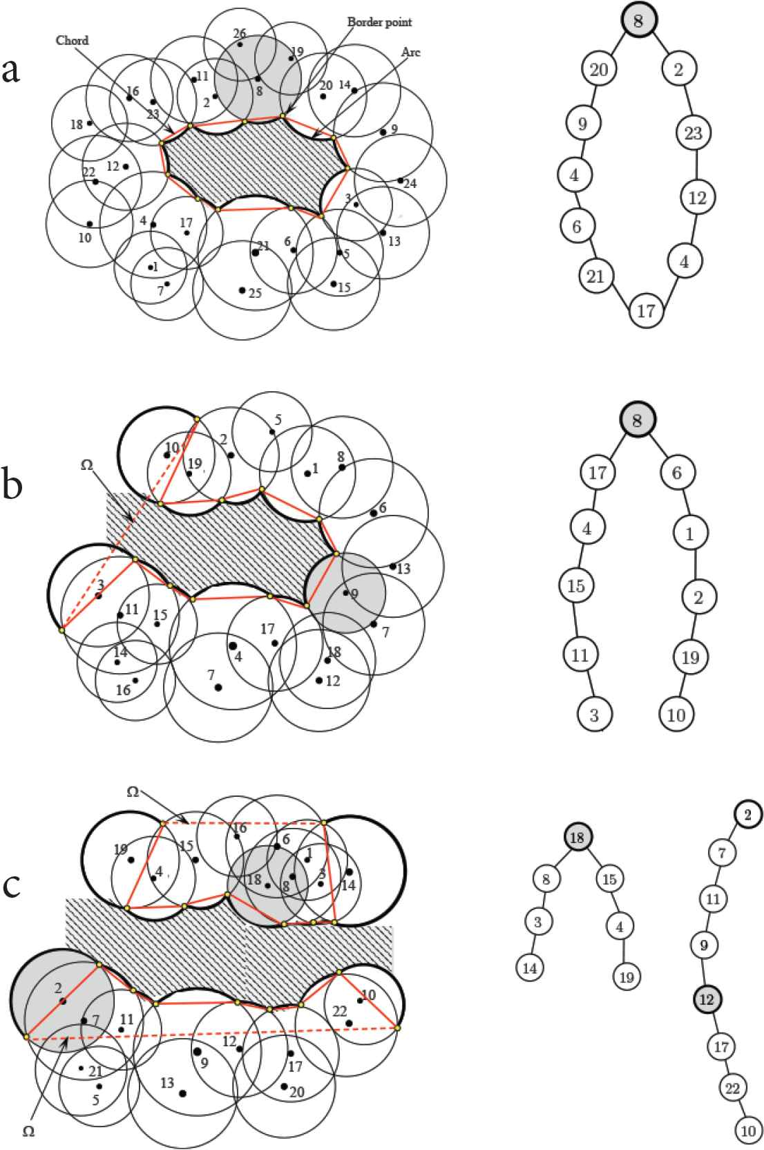
Different types of holes and their corresponding graphs of parents: (a)–(c) on left gray node is the initiator, on right gray node is the coordinator.
The coordinator will be chosen by the initiator using the graph of parents denoted by Gp = (Vp, Ep) built from the border points (see Definitions 3 and 4) contained in ARC messages.
The graph of parents induces a ring (cycle), a tree or a chain (path) when the coverage hole is respectively closed or open. Coordinator election process complies with the following rules:
- •
if this graph is cyclic (see Theorem 1) the initiator becomes the coordinator;
- •
otherwise, the initiator is the root of a tree containing two sets of nodes or branches denoted by b1 and b2 such as |b2| ≥ |b1| with |b2| > 0 and |b1| ≥ 0; then the node located
After choosing another node as a coordinator, the initiator must send a COORD message containing information needed to conduct the coverage recovery process such as the uncovered arcs, the type of topology induced by the detected coverage hole, and information that help to update the timer talert of all the nodes that have entered into Alert state.
The coverage recovery process is started by the coordinator just after its election upon receiving a COORD message or directly, if it was the former initiator.
3.3.3. Hole elimination phase
The entire coverage recovery process is supervised by the coordinator. This process consists of three phases, namely: relocation sites definition, candidates selection, and candidates migration.
• Relocation sites definition
This phase starts with the location of hole H’s centroid denoted by G. To do this, coordinator must find the set of border points starting by the ones located on its own perimeter. These points will be referred to as pi in the remainder of this description; i denotes the index granted by the coordinator. The latter gets each border point pi’s coordinates respectively denoted by xi and yi from information contained in the uncovered arcs.
When the hole is closed, point G corresponds to the barycenter of the irregular polygon induced by its convex hull. G’s coordinates respectively denoted by xG and yG, are calculated using Equations (4)–(6).
However, if hole H is open, G is located such as
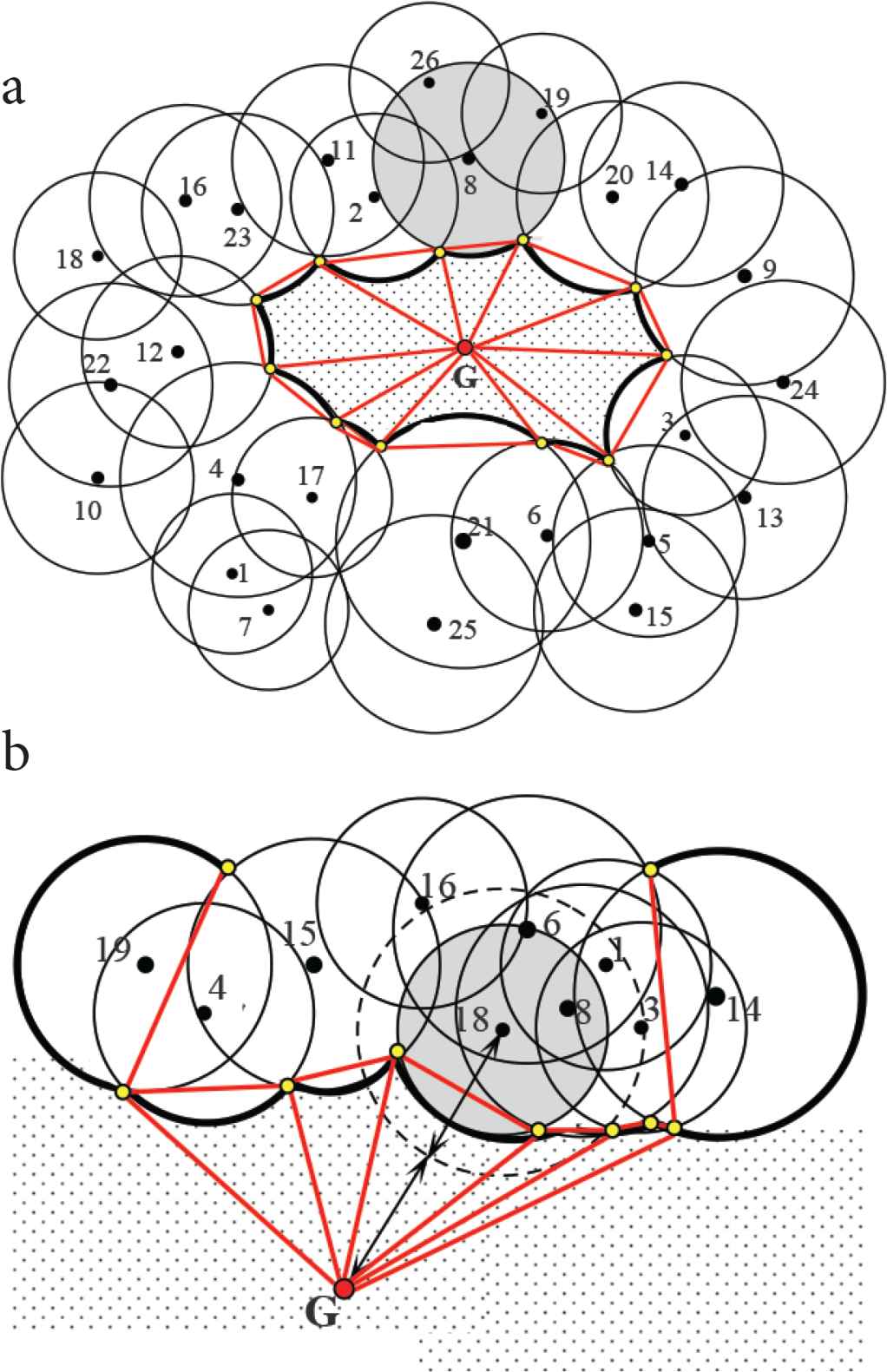
Hole discretization by a coordinator (in gray): (a) hole is closed (b) hole is open.
After locating the centroid G, coordinator u must discretize hole H linking each border point pi to G. Figure 3a and 3b depict results respectively obtained with a closed hole and an open one.
Each resulting triangle will be referred to as a zone in the remainder of this description. coordinator u must also determine inside hole H all the relocation sites. To do this, each segment
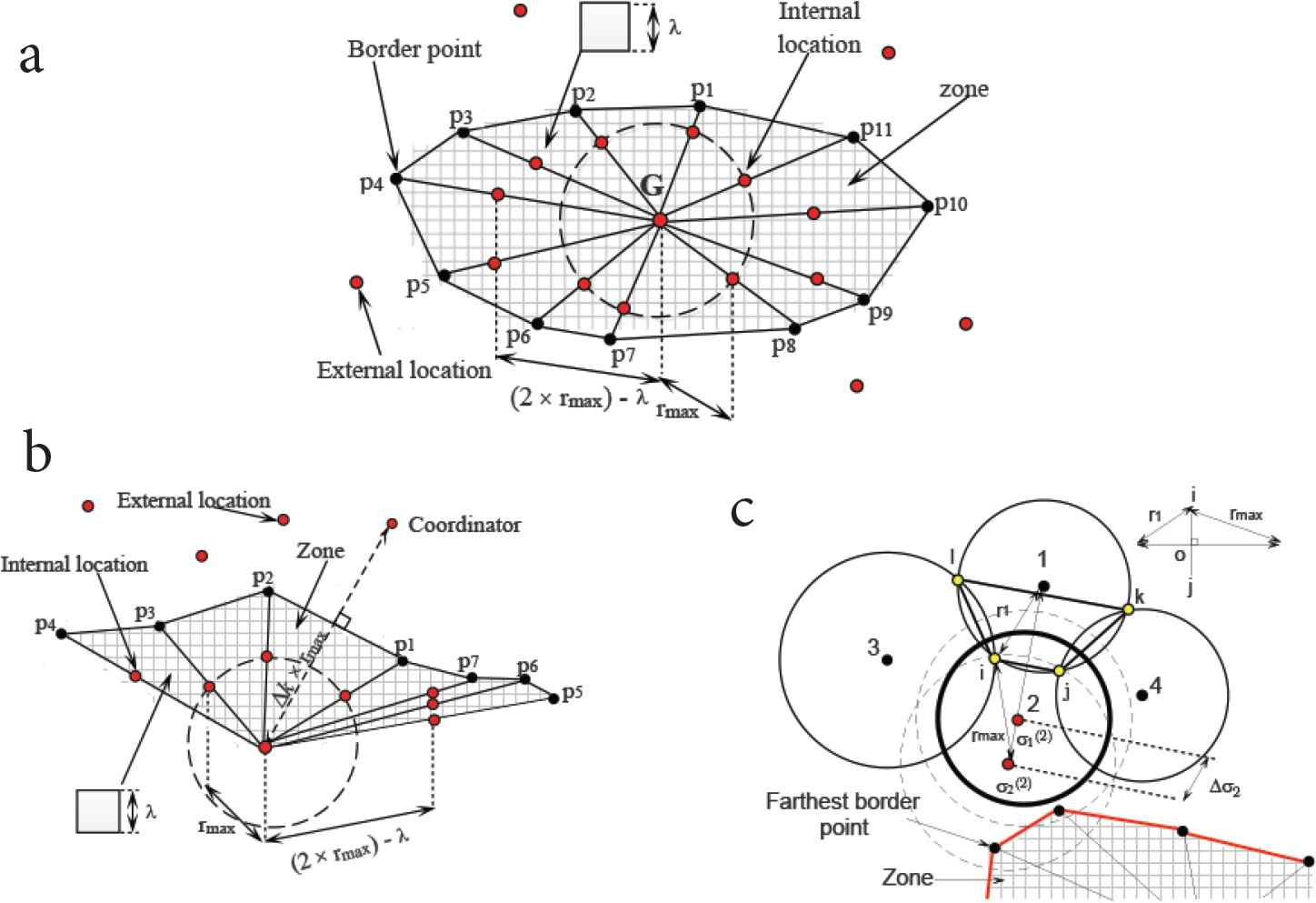
Finding potential positions (in red): (a) by the coordinator for a closed hole (b) by the coordinator for an open hole (c) by a potential candidate (Virtual grid is only used to estimate the coverage ratio in each zone. See online version for colors).
After hole discretization process, coordinator u broadcasts in its two-hop neighborhood a SITE message containing information about the border points and those located inside hole H. Then, it starts a timer whose duration tsite(u) is initiated using the maximum round trip time experienced among its neighbors. This timer is updated using Equation (7) upon receiving any response (CANDIDATE message) from a neighbor v.
τ(i,i+1) denotes the transmission delay between two consecutive nodes on the path between nodes u and v. rtt(v) is the maximum round trip time between node v and its neighbors. π(u, v) is the set of intermediary nodes on the path between u and v.
Upon receiving a SITE message, any node v in Alert state must define its elbow room Φ(v) (see Definition 7). Indeed, in coordinator u’s two-hop neighborhood each node v must find with respect to each of its own neighbors, the farthest external position denoted by
The farthest position found with respect to neighbor 1 requires node 1, 3, and 4 to be immobilized (i.e. η(μ) = {1, 3, 4}). Note that node 2 has also found that choosing its current position as a potential relocation site does not require any neighbor to be immobilized (i.e. η(u) = ∅).
Node 2 will try to do the same with each of its other neighbors located further away with respect to G. Therefore, Node 2’s elbow room is the set of actions to perform in order to reach the hole without compromising its coverage. Redundant potential candidates generally have the largest rooms for maneuver. Indeed, such nodes can freely move toward several sites (external or not) without compromising deployment zone coverage. To do this, these nodes must select sites (especially the internal ones) by immobilizing their neighborhood; knowing that a node may be redundant with respect to different subsets of neighbors. For example, in Figure 5a node 1 (in gray) is redundant with respect to two subsets of neighbors namely {2, 3, 5, 6} and {2, 3, 4, 5, 6}; therefore, any displacement toward a site will require node 1 to immobilize only the smallest set of neighbors namely, {2, 3, 5, 6} (i.e. η(μ) = {2, 3, 5, 6}). In Figure 5b node 1 and node 4 are respectively redundant in relation to {2, 3, 5, 6} or {2, 3, 4, 5, 6} and {5, 6, 7, 8, 9}. Therefore, the two subsets of neighbors to be immobilized during the displacements of node 1 and node 4, are respectively {2, 3, 5, 6} and {5, 6, 7, 8, 9}.
Neighbors immobilization process by a redundant candidate (in gray): (a) with multiple redundancy neighborhood. (b) with a redundant neighbor.
Note that like any potential candidate, redundant nodes must make sure that they have enough energy to move to any selected site and reach at least one zone from that position (see Definition 6).
Also note that any area coverage redundancy check protocol found in the literature can be used to detect redundant nodes [14]. Although, we suggest the MRZ-based one we proposed in our previous works [51,52].
If a node v has a sufficient elbow room (i.e. Φ(v) ≠ ∅) it becomes a formal candidate by sending CANDIDATE message to the coordinator and starts a timer for tcand (v) units of time. This message contains information about its elbow room, and state. tcand (v) is estimated using Equation (13) in terms of the round trip time on the path π(u, v) between v and coordinator u. The latter information is contained in the SITE message sent by the coordinator.
From mobility point of view, there are three types of formal candidates (with respect to their states) which might be involved in the coverage recovery process namely: nodes that are unable to move, nodes with reduced mobility, and those with full mobility. These types of candidacy respectively correspond to intermediary states MO, MRM, and MM. Note that coordinator may be a candidate as well.
≠ Candidates selection
This last phase allows coordinator u to ensure coverage recovery optimization. Indeed, after timer tsite(u) expiration, coordinator u must choose the maneuvers which help to best eliminate the hole while minimizing overlapped areas and energy wastes.
We formulate this issue as a location-allocation problem [20,21]. The latter has several well-known variants in combinatorics and geometry (facility location, p-median, p-center, set covering, Weber problem...) [53,54].
Solutions commonly proposed in the literature have many applications in domains such as industry, geography, transportation, logistics, marketing etc. We formulate this problem using the following mixed integer linear program:
Let xij be the area exclusively covered in zone j by the candidate involved in maneuver i. Let
s.t.:
Equation (14) states the objective namely, minimize the uncovered areas, the overlapped areas inside the hole and the total energy consumption. Equation (15) states that each zone j must be entirely covered. Equation (16) suggests that any maneuver i should reach at least one zone j. This constraint ensures that each candidate is active and is able to reach at least one zone. Equation (17) ensures that the residual energy of the candidate concerned by a maneuver is enough if allowed. Equation (18) prevents coordinator to allow incompatible maneuvers. This constraint prevents illogic maneuvers (ubiquity), new hole formation, collisions, and oscillations. Equation (19) ensures that any solution allows at least one maneuver. Equations (20)–(22) define the decision variables. Equations (23)–(25) define the constants.
Energy costs are calculated using Equation (26); where εdist(.) and εrange(.) are two functions respectively related to the underlying mobility and motility energy consumption models. Er(v) is the residual energy of the candidate v concerned by maneuver i.
Note that in practice, it is difficult to comply with the constraint suggested by Equation (15) since nodes are randomly deployed and their density constantly decreases. Therefore, coordinator can relax Equation (15) by Equation (27) if n < ψ*; where n denotes the numbers of available redundant candidates whereas ψ* denotes the maximum number of candidates required to totally cover hole H; its value is obtained using Equation (28) inspired from Tóth [55]; where
Any method of the literature can be used to estimate the area of hole H. As suggested by Figure 4a and 4b, an intuitive method is to add up the calculated areas (e.g. using Heron’s formula) of the zones (triangles) created during the hole discretization process. For closed holes,
According to a method commonly used in the literature dj, xij and ϕij can be estimated by discretizing each zone j with a virtual grid of patterns such as points, squares etc. [56–58]. Figure 6 illustrates how to estimate these values. Let j (in red) be a zone of a detected hole discretized with a grid of 24 cells (dj = 24). In this example, we consider that a cell is entirely covered by a node if its four corners are within the node’s range (i.e located at a distance inferior or equals to the circle’s radius). r, s, t, u, v, w denote six nodes that can reach zone j. Node r exclusively covers six cells (namely cells 3, 4, 5, 9, 10, and 11); node s covers cells 19 and 20; node t cells 15, 21, and 22; node u cells 1, 7, 8, and 13; node v cell 2. Instead, node w does not exclusively cover any cell. Therefore, xrj = 6, xsj = 2, xtj = 3, xuj = 4, xvj = 1, xwj = 0. Nodes r, s, u yield no overlapped areas; instead, node t yields overlapped area in cell 20, node v in cells 1, 7, and 8; node w in cells 13, 19 and 20. Therefore, ϕrj = 0, ϕsj = 0, ϕtj = 1, ϕuj = 0, ϕvj = 3, ϕwj = 3.
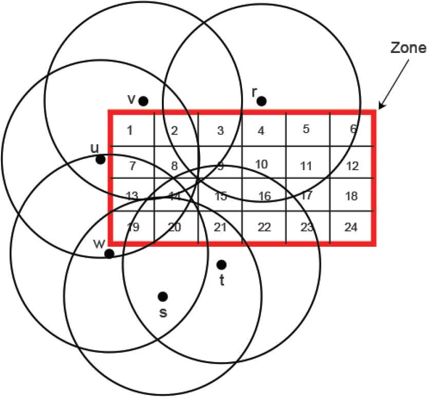
Exclusive and overlapped area coverage estimations in a virtual grid-based discretized zone.
Note that, in this example we have discretized zone j with large squares only to simplify our explanations. One could also have used smaller grid cells or even points [57] to increase precision and minimize estimation errors like those yielded by coverage in cells 14 and 16.
Coordinator defines incompatibilities zij between two maneuvers i and j with respect to their origins (ubiquity), destinations (collision) or immobilizations contained in candidates’ elbow rooms (see Definitions 7 and 10)
Regrettably, location-allocation problem has been proven NP-hard [59–61]. Therefore, we propose an approximate solution based on tabu search metaheuristic [62].
A local reorganization scheme s (i.e. a simplified version of a feasible solution) will denote a set of n maneuvers, each related to a unique candidate. Formally, s = {i ∈ I: yi = 1} with |s| = n. To find an initial solution, coordinator first looks for the best (i.e. less energy consuming) maneuver toward the centroid; then, if found, allows it and store the concerned candidate’s identifier.
For each candidate v (except the one eventually sent to the centroid), coordinator will look for all the maneuvers of v that are compatible with the ones already allowed. If v is redundant then coordinator chooses the most energy consuming maneuver of v; otherwise, the less energy consuming one. The set of all maneuvers thus allowed will be referred to as the initial local reorganization scheme.
During the optimal local reorganization scheme search process, neighbor solutions will be obtained by shifting two maneuvers.
During the decision making process, coordinator will use candidates’ maximum range denoted by
A local reorganization scheme s = {i1, i2, …, in} corresponds to decisions made by coordinator for each of the n candidates taking account of maneuvers’ incompatibilities. For instance, applying a move on i1 consists in finding for the concerned candidate a new maneuver
• Candidates migration
After finding an optimal local reorganization scheme, coordinator u broadcasts a MOVE message containing its decisions. Upon receiving such a message, candidates start moving to their new relocation sites. MOVE messages are forwarded via paths used by SITE messages.
Nodes will optimize their ranges using any scheme of the literature [63–65] upon reaching destination and timer tmove (u) expiration. Redundant nodes will eventually enter into sleep state.
Figure 7 depicts the rationale behind CHEAP. Figure 8 shows the state diagram of the discussed coverage hole detection and elimination schemes.
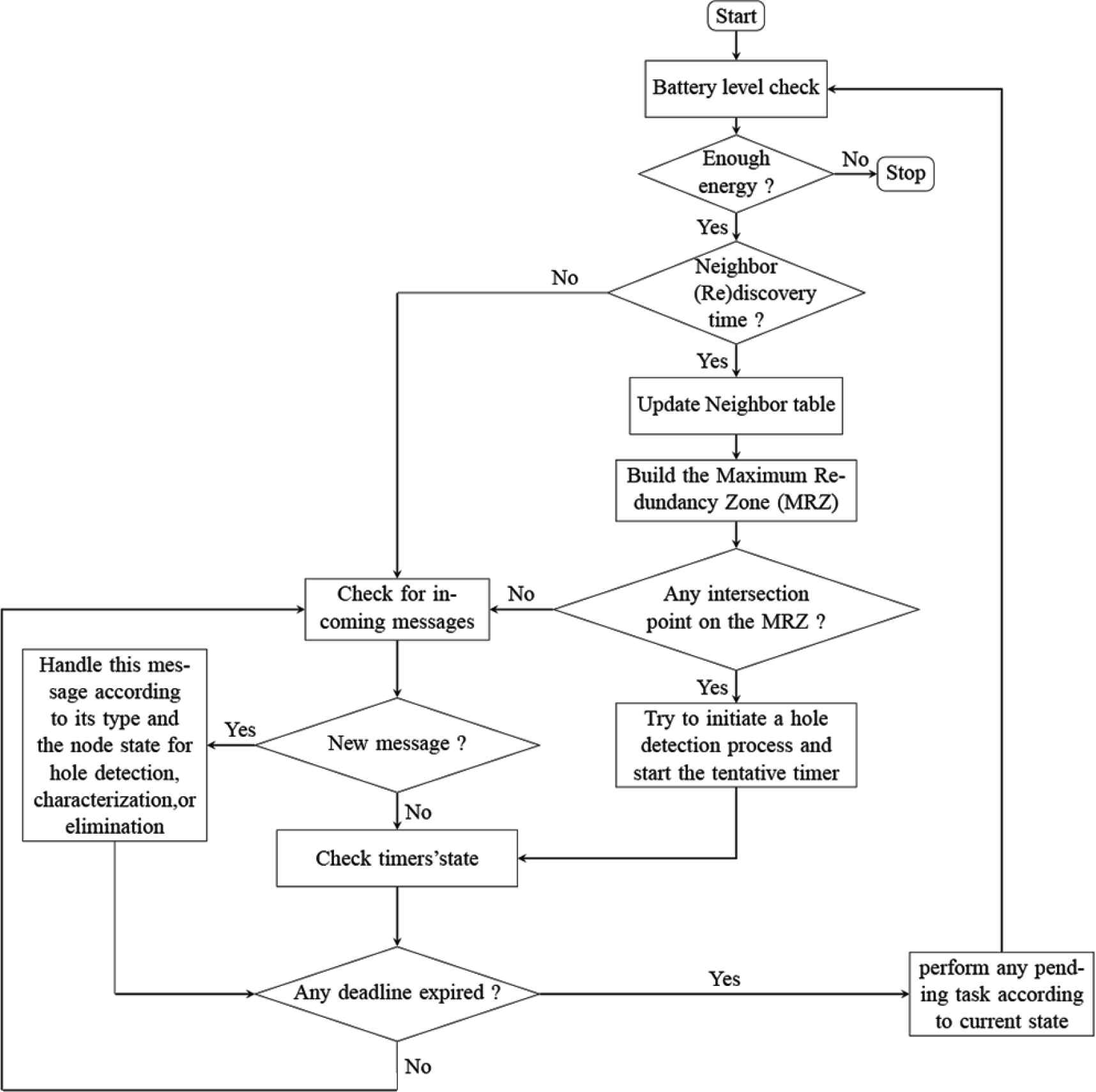
Flowchart of CHEAP.
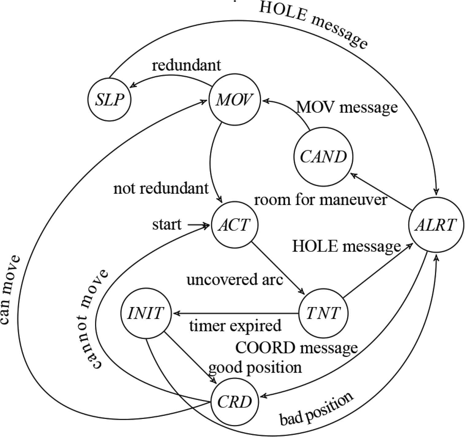
State diagram of CHEAP.
Table 1 summarizes the variables used in the different algorithms.
| Name | Definition |
|---|---|
| crd(u) | coordinator of the hole elimination process involving node u |
| D | set of relocation sites inside a hole |
| deadline | current deadline of a timer |
| dest(u) | destination node u is allowed to move to |
| Δk | range offset for open hole’s centroid |
| Ea(u) | set of edges between arcs’ parents discovered by node u |
| Er(u) | node u’s residual energy |
| Eth | residual energy threshold |
| G | centroid of a hole |
| Φ(u) | set of maneuvers that node u can perform (its elbow room) |
| I | set of candidates’ maneuvers |
| idu | node u’s identifier |
| init(u) | initiator of the hole detection process involving node u |
| IP(u) | intersection points between node u and its neighbors |
| IN(u) | intersection points between node u’s neighbors |
| itmax | maximum number of iterations |
| J | set of sub-areas inside a hole (zone) |
| K | set of nodes’ sensing ranges |
| λ | length of a virtual grid cell |
| ls | size of the tabu list |
| MRZ(u) | set of points on the convex’s hull of node u’s MRZ (see Definition 9) |
| N(u) | node u’s neighbor table |
| NH(u) | set of candidates for the coverage recovery process led by node u |
| η(u) | node u’s immobilized neighborhood (see Definition 7) |
| P | set of points on hole’s border |
| rs(u) | current sensing range of node u |
|
|
maximum sensing range |
| rtt(v) | round trip time with neighbor v |
| s* | optimal reorganization scheme |
| state(u) | current state of node u (see Definition 11 for possible values) |
| Sr(u) | set of uncovered arcs so far reported by node u |
| talert(u) | duration of node u’s on alert state |
| tcand(u) | duration of node u’s candidate state |
| tdiscov | duration between two neighbor (re)discovery periods |
| tinit(u) | duration of node u’s initiator state |
| tmax | maximum duration of tentative state |
| tmov(u) | duration of node u’s on move state |
| tsite(u) | duration of node u’s coordinator state |
| tsleep(u) | duration of node u’s sleep state |
| ttent(u) | duration of node u’s tentative state |
| ϒij | set of parents of points i and j (see Definition 3) |
| Va(u) | set of arcs’ parents |
| χ(i) | parents of point i (see Definition 3) |
| xG | abscissa of the hole’s centroid |
| yG | ordinate of the hole’s centroid |
Main global variables
Algorithms 1–4 formally describe coverage hole detection, characterization, and elimination processes. Algorithms 5 and 6 specifically describe the optimal local reorganization scheme search process.
| Require: Er(u), Eth, tdiscov, tmax, K, ls, deadline, Δk... ⊳ see Table 1 |
| 1: Er(u)← get_residual_energy() ⊳ check battery level |
| 2: while (Er(u)>Eth) do ⊳ is residual energy enough ? |
| 3: if ((current time() = delay_DISC)) then |
| 4: if (state(u) = ACT) then |
| 5: N(u) ← neighbor_discovery() |
| 6: IP(u) ← get_points_with_neighbors (N(u)) |
| 7: IN(u) ← get_points_among_neighbors (N(u)) |
| 8: MRZ(u) ← get_MRZ_hull (IN(u), IP(u), N(u)) |
| 9: if ((IP(u) ∩ MRZ(u)) ≠ ∅) then ⊳ found uncovered arcs |
| 10: state(u) ← TNT |
| 11: ttent(u) ← random_uniform ([0; tmax]) |
| 12: deadline ← current_time() + ttent(u) |
| 13: end if |
| 14: end if |
| 15: delay_DISC ← current_time() + tdiscov |
| 16: end if |
| 17: receive message from v ⊳ new message from a neighbor v |
| 18: switch message do |
| 19: case HOLE |
| 20: |
| 21: ϒij ← get_parents ( |
| 22: if (state(u) ∈ {ACT, TNT, SLP})∧(idu ∈ ϒij) then |
| 23: IP(u) ← get_points_with_neighbors (N(u)) |
| 24: IN(u) ← get_points–among–neighbors (N(u)) |
| 25: MRZ(u) ← get_MRZ_hull (IN(u), IP(u), N(u)) |
| 26: |
| 27: rs(u) ← |
| 28: state(u) ← ALRT |
| 29: init(u) ← message.init ⊳ initiator’s id |
| 30: if ( |
| 31: talert(u) ← get_path_delay (message) |
| 32: deadline ← current_time() + talert(u) |
| 33: send HOLE(init(u), |
| 34: send ARC({ |
| 35: else |
| 36: forward_or_delete (message, N(u), v, ttlmax) |
| 37: end if |
| 38: else |
| 39: forward_or_delete (message, N(u), v, ttlmax) |
| 40: end if |
| 41: case ARC |
| 42: if ((state(u) = INIT)∧(message.init = init(u))) then |
| 43: { |
| 44: tinit(u) ← get_path_delay (message) |
| 45: deadline ← deadline + tinit(u) |
| 46: Va(u) ← (Va(u)\{ |
| 47: Ea(u) ← Ea(u) ∪ { |
| 48: else |
| 49: forward_or_delete (message, N(u), v, ttlmax) |
| 50: end if |
| 51: otherwise |
| 52: elimination (message, v, IP(u), ...) ⊳ see Algorithm 2 |
| 53: end switch |
| 54: detection_timers (IP(u), IN(u), ...) ⊳ see Algorithm 3 |
| 55: elimination_timers (IP(u), IN(u), ...) ⊳ see Algorithm 4 |
| 56: Er(u) ← get_residual_energy() ⊳ check battery level |
| 57: end while |
Hole detection process by a node u
| Require: message, v, IP(u), MRZ(u), deadline, ... ⊳ see Table1 |
| 1: switch message do |
| 2: case COORD |
| 3: if (state(u) = ALRT)∧(message.coord = idu)) then |
| 4: P ← find_border_points (Va(u), Ea(u)) |
| 5: G ← get_centroid (P, Δk) ⊳ Equations (4) and (5) |
| 6: J ← triangulation (P, G) ⊳ Hole discretization |
| 7: create_virtual_grid (J) |
| 8: D ← set_internal_sites(P, |
| 9: state(u) ← CRD |
| 10: send SITE(D, P) to w, ∀w ∈ N(u)\v |
| 11: tsite(u) ← max{rrt(v), ∀v ∈ N(u)} |
| 12: deadline ← current_time() + tsite(u) |
| 13: Φ(u) ← get_elbow_room (D, P) |
| 14: message.ttl ← ttlmax |
| 15: end if |
| 16: case SITE |
| 17: if ((state(u) = ALRT)∧(message.init = init(u))) then |
| 18: Φ(u) ← get_elbow_room (message.D, message.P) |
| 19: if (Φ(u) ≠ ∅) then |
| 20: send CANDIDATE (Φ(u), message.coord) to v |
| 21: state(u) ← CAND |
| 22: tcand(u) ← get_path_delay (message) |
| 23: deadline ← current_time() + tcand(u) |
| 24: end if |
| 25: end if |
| 26: case CANDIDATE |
| 27: if ((state(u) = CRD)∧(message.init = init(u))) then |
| 28: D ← D ∪ get_external_locations (message) |
| 29: I ← I ∪ get_travel_paths (message) |
| 30: NH(u) ← NH(u) ∪ {v} |
| 31: tsite(u) ← get_path_delay (message) |
| 32: deadline ← deadline + tsite(u) |
| 33: message.ttl ← ttlmax |
| 34: end if |
| 35: case MOVE |
| 36: if ((state(u) = CAND)∧(message.init = init(u))) then |
| 37: d ← get_new_location (message.s*) |
| 38: state(u) ← MOV |
| 39: tmov(u) ← get_travel_time (d) |
| 40: travel to d |
| 41: deadline ← current_time() + tmov(u) |
| 42: end if |
| 43: end switch |
| 44: forward_or_delete (message, N(u), v, ttlmax) |
Hole elimination process by a node u
| Require: IP(u), MRZ(u), Va(u), Ea(u), deadline, Δk ... ⊳ see Table 1 |
| 1: if (current_time() = deadline) then |
| 2: switch state(u) do |
| 3: case TNT |
| 4: Cr ← get_arcs (IP(u)∩MRZ(u)) |
| 5: for all |
| 6: |
| 7: end for |
| 8: Nr ← argmin ( |
| 9: |
| 10: send HOLE ( |
| 11: state(u) ← INIT |
| 12: tinit(u) ← max{rrt(v), ∀v ∈ N(u)} |
| 13: deadline ← current_time() + tinit(u) |
| 14: Sr(u) ← Sr(u) ∪ { |
| 15: case INIT |
| 16: if (Va(u) ≠ ∅) then |
| 17: Vp ← get_parents (Va(u)) |
| 18: Ep ← link_between_parents (Ea(u)) |
| 19: crd(u) ← find_coordinator (Vp, E p) |
| 20: if (crd(u) = idu) then |
| 21: P ← find_border_points (Va(u), Ea(u)) |
| 22: G ← get_centroid(P, Δk) ⊳ Equations (4) and (5) |
| 23: J ← triangulation(P, G) |
| 24: create_virtual_grid(J) |
| 25: D ← set_internal_sites(P, |
| 26: state(u) ← CRD |
| 27: send SITE(D, P) to w , ∀w ∈ N(u)\v |
| 28: tsite(u) ← max{rrt(v), ∀v ∈ N(u)} |
| 29: deadline ← current_time() + tsite(u) |
| 30: Φ(u) ← get_elbow_room(D, P) |
| 31: else |
| 32: if ((Va(u) ≠ ∅)∧(Ea(u) ≠ ∅)) then |
| 33: send COORD(Va(u), Ea(u)) to crd(u) |
| 34: state(u) ← ALRT |
| 35: end if |
| 36: end if |
| 37: else |
| 38: state(u) ← ACT |
| 39: init(u) ← 0 |
| 40: end if |
| 41: case ALRT |
| 42: state(u) ← ACT |
| 43: init(u) ← 0 |
| 44: end switch |
| 45: end if |
Detection timers check for a node u
| Require: I, J, D, NH(u), itmax, ls, deadline, s* .... ⊳ see Table 1 |
| 1: if (current_time() = deadline) then |
| 2: switch state(u) do |
| 3: case CRD |
| 4: s* ← reorganization (I, J, K, ..) ⊳ see Algorithm 5 |
| 5: if (s* ≠ ∅) then |
| 6: send MOVE (s*) to v, ∀v ∈ NH(u) |
| 7: end if |
| 8: if (Φ(u) ≠ ∅) then |
| 9: d ← get_new_location(s*) |
| 10: state(u) ← MOV |
| 11: tmov(u) ← get_travel_time(d) |
| 12: travel to d |
| 13: deadline ← current_time() + tmov(u) |
| 14: end if |
| 15: case CAND |
| 16: state(u) ← ACT |
| 17: case MOV |
| 18: rs(u) ← get_new_range(s*) |
| 19: if (check_redundancy()) then |
| 20: state(u) ← SLP |
| 21: tsleep(u) ← get_sleep_time() |
| 22: deadline ← current_time() + tsleep(u) |
| 23: else |
| 24: state(u) ← ACT ⊳ return to normal state |
| 25: optimize_range() ⊳ see [63–65] |
| 26: end if |
| 27: case SLP |
| 28: state(u) ← ACT ⊳ return to normal state |
| 29: end switch |
| 30: end if |
Elimination timers check for a node u
| Require: I, J, D, G, K, NH(u), itmax, ls, s* |
| 1: s ← get_initial_solution(I, K, G, NH(u)) ⊳ see Algorithm 6 |
| 2: s* ← s |
| 3: LT ← ∅ ⊳ tabu list initialization |
| 4: nitr ← 0 |
| 5: while (nitr < itmax) do |
| 6: N(s) ← {s′ |are_neighbors(s′, s)∧(s′ ∉ LT)} : |N(s)| ≤ ls |
| 7: δ ← 1 |
| 8: if (N(s) ≠ ∅) then |
| 9:
|
| 10: if ( f(
|
| 11: s* ← |
| 12: end if |
| 13: update_list (LT, N(s)) |
| 14: δ ← |N(s)| |
| 15: else |
| 16: s ← argmin (f(s′)) ⊳ aspiration s′∈LT |
| 17: LT ← LT\s |
| 18: end if |
| 19: nitr ← nitr + δ |
| 20: end while |
Tabu-based optimal reorganization scheme search
| Require: I, K, G, NH(u) |
| Ensure: s |
| 1: k ← max(K) ⊳ use maximum sensing range |
| 2: Λ ← argmax (check_destination(i, G))i∈I |
| 3: C* ← ∅ |
| 4: if (Λ ≠ ∅) then |
| 5: i* ← argmin (ɛ dist(i)) i∈Λ |
| 6: |
| 7: s ← s ∪ {(i*; k)} ⊳ update the solution |
| 8: C* ← get_candidate_id(i) ⊳ get the node involved |
| 9: end if |
| 10: for all v ∈ NH(u)\C* do |
| 11: ϒ ← argmax (check_origin(i, v) + compatible (i, |
| 12: if (ϒ ≠ ∅) then |
| 13: if (is_movable(v)) then ⊳ can v move ? |
| 14: i* ← argmax (ɛ dist(i)) ⊳ assign the farthest maneuver i∈ϒ |
| 15: else |
| 16: i* ← argmax (ɛ dist(i)) ⊳ assign the nearest maneuver i∈ϒ |
| 17: end if |
| 18: |
| 19: s ← s ∪ {(i*; k)} ⊳ update the solution |
| 20: end if |
| 21: end for |
| 22: return s |
Initial reorganization scheme generation by a coordinator u
4. PERFORMANCE EVALUATION
In order to verify and validate our scheme, we chose OMNeT++ 5.5 simulator [66] to evaluate our solution with respect to different metrics. Results are compared to those obtained with three major related protocols proposed in the literature: DECM by Qiu and Shen [40], HORA by Sahoo and Liao [39], and ZBFR by Sharma and Sharma [18].
We used the communication and the sensing energy consumption models respectively proposed by Heinzelman et al. [67] and by Halgamuge et al. [68]. We also used a mobility energy consumption model [see Equations (29)–(33)] inspired from the method proposed by Society of Robots [69].
Since this process is supposed to take place in the plan (see Section 3.2), potential energy is null ((Ep = 0) ⇔ (h = 0)).
For each experiment, we deployed several networks; each of them is composed of randomly and uniformly distributed nodes. To randomly vary the average times between two consecutive faults, we used the Weibull distribution combined with the Uniform distribution as described in Table 2. Faults were injected using these factors under an unfair distributed daemon.
| Factors | Unit/Description | – | + |
|---|---|---|---|
| Fault scale* | Area of the hole |
|
|
| MTBF** | Average time between two faults |
|
|
| Fault effect*** | Degree of severity | 0 |
|
Value to square; unit is m2.
(Mean Time Between Failures) expressed in seconds (simulated time).
nodes displacement = 0, damaged sensing unit = 1, node failure = 2.
Fault tolerance factors
Fault injection consisted in randomly constructing an irregular polygon so that only intersecting nodes experience a fault (displacement or failure). Note that battery exhaustion is only due to energy losses and self-discharge.
In the following sections, we first detail all the experiments we have conducted. Then we analyze and explain their results. In the course of these experiments we evaluated the impact of the factors described in Table 2 on the selected metrics. Note that each experiment was repeated 100 times. The results were obtained with a 95% confidence interval. The simulation parameters are summarized in Table 3.
| Parameter | Value |
|---|---|
| Deployment area | 1000 m × 1000 m |
| Number of sensors | 100 to 1000 |
| Sink’s position | (450;200) |
| Sensors’ communication ranges | {15;35;54;70;83;98;117;127} m |
| Sink’s communication range | 250 m |
| Sensors’ initial energy (Ei) | 2.5 J |
| Self-discharge per second | 0.1 μJ |
| Threshold energy (Ethr) | 100 μJ |
| Eelec | 50 nJ/bit |
| efs | 10 nJ/bit/m2 |
| eamp | 0.0013 nJ/bit/m4 |
| d0 | 87 m |
| Message length (l) | 2000 bits |
| ttlmax | 2 |
| Usup | 2.7 V |
| Isens | 25 mA |
| tsens | 0.25 ms |
| Data size(b) | 200 bits |
| Mass (m) | 0.5 kg |
| Maximum velocity (v) | 0.06 m/s |
| Deceleration rate (
|
|
| Chemical efficiency (ea) | 90% |
| Mechanical efficiency (eb) | 70% |
| Electrical efficiency (ec) | 95% |
| Thermal efficiency (ed) | 100% |
| Virtual grid cell length (λ) | 7 m |
| Range offset (Δk) | 3 |
| Maximum number of iterations (itmax) | 200 |
Simulation parameters
4.1. Average Hole Detection Time
During this experiment, when a fault was injected, simulation daemon recorded the occurrence time, hole localization, and information about boundary nodes. Hole detection time was determined by the simulation program after having received a signal from all the boundary nodes. The resultant detection times were averaged at the end of the simulation (i.e. after all sensors died). Note that detection time of an undetected hole was obtained by subtracting the fault injection time from the simulation duration.
Figure 9a and 9b suggest that for all the evaluated protocols, average hole detection time increases according to network size and fault scale. However, CHEAP provides the lowest detection times. These results are essentially due to the fact that, unlike other protocols, CHEAP does not define waiting times according to nodes’ degrees. Indeed, to avoid endless edge flipping during the Delaunay triangulation, DECM sets a timer which depends on nodes’ degrees; while the performance of HORA is due to the mobility invitation messages sent. ZBFR yields the worst times because of the heartbeat message used for large agreement regions as well as for failures involving the Zone Monitor.
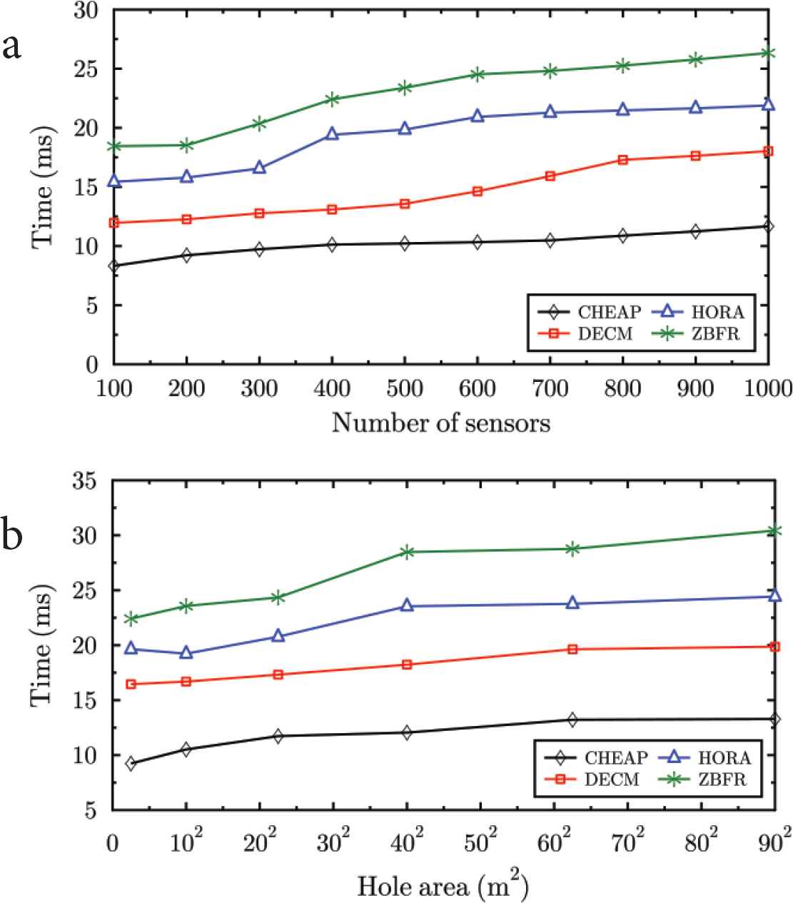
Average hole detection time: (a) Impact of network size; (b) Impact of fault scale for network size = 1000.
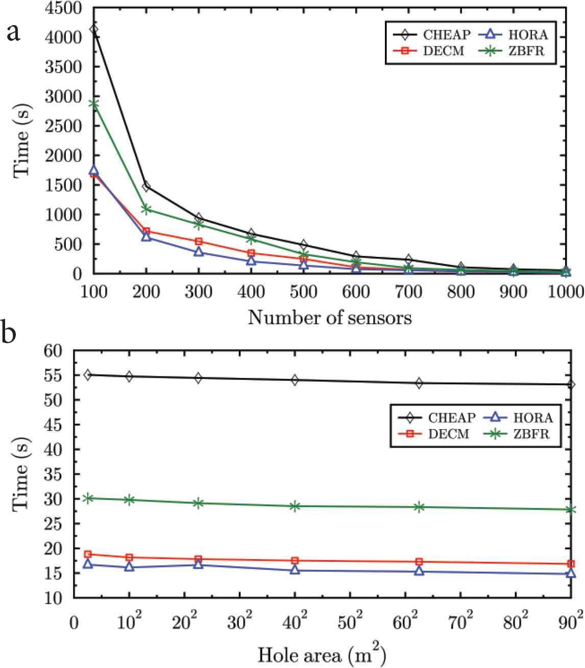
4.2. Average Hole Elimination Time
In this experiment, hole elimination time was determined by the simulation program after having received a signal from all the candidates when reaching their final destinations. The resultant elimination times were averaged after all sensors died. Note that the elimination time of an uncovered hole was obtained by subtracting the fault injection time from the simulation duration.
Figure 10a and 10b shows that average hole elimination time increases according to network size and fault scale when using all the evaluated protocols. However, CHEAP provides the lowest values, i.e. approximately half the times obtained with the other evaluated protocols. This is due to CHEAP’s ability to avoid nodes’ cascaded movements which increase the coverage recovery process’ latency. This is particulary true with DECM whose hole elimination time suffers from the cooperative movement scheme proposed by its authors. Performance of HORA is also due to the delay induced by the nodes’ mobile region and the nearest assistant node selection processes. As for ZBFR, its back up nodes designation process (sleeping nodes activation + redundancy check + sleep rescheduling) conducted by the Zone Monitors contributes to increasing hole elimination delay.
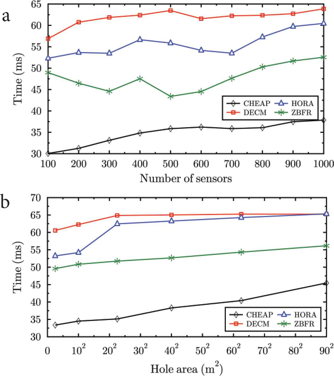
Average hole elimination time: (a) effect of network size; (b) effect of fault scale for network size = 1000.
4.3. Average Mobilization Ratio
This experiment was aimed to evaluate each protocol’s ability to minimize the number of candidates required to eliminate a hole. To do this, the simulation program recorded the set of potential candidates located two hops from the hole created after fault injection. After hole elimination, the simulation program calculated the ratio between the number of potential candidates and the number of candidates actually used.
After the last sensor died, the experiment was stopped and the resulting ratios were averaged. Figure 11a and 11b respectively suggest that regardless of the protocol evaluated, average mobilization ratio decreases while the network size grows but increases according to fault scale. Intuitively, the higher is the node density the lower is the number of candidates to be relocated. On the other hand, the larger is the coverage hole, the higher will be the number of required candidates. HORA yields the highest ratios (60–55%) especially when the number of sensors is large. Indeed, the mobility invitation-based scheme used in HORA tends to move all the possible candidates, even when the hole is already eliminated. The performances of DECM are more mitigated with an average ratio of 45% when the network size is 1000 and the hole area is 90 × 90 m2. This is due to the cooperative movement mechanism applied in DECM to prevent generating new holes during node movements. Indeed, this strategy can lead to cascaded movements especially when node density is low. On the contrary, the strategy based on nodes’ redundancy and mobility helps ZBFR to better cope with these cascaded movements, the low average ratios we obtained (50–42%). A similar strategy was applied in CHEAP; however, the node motility (i.e. range control) scheme helps to better minimize the number of moving candidates; hence, the lowest ratios (i.e. 40–35%).
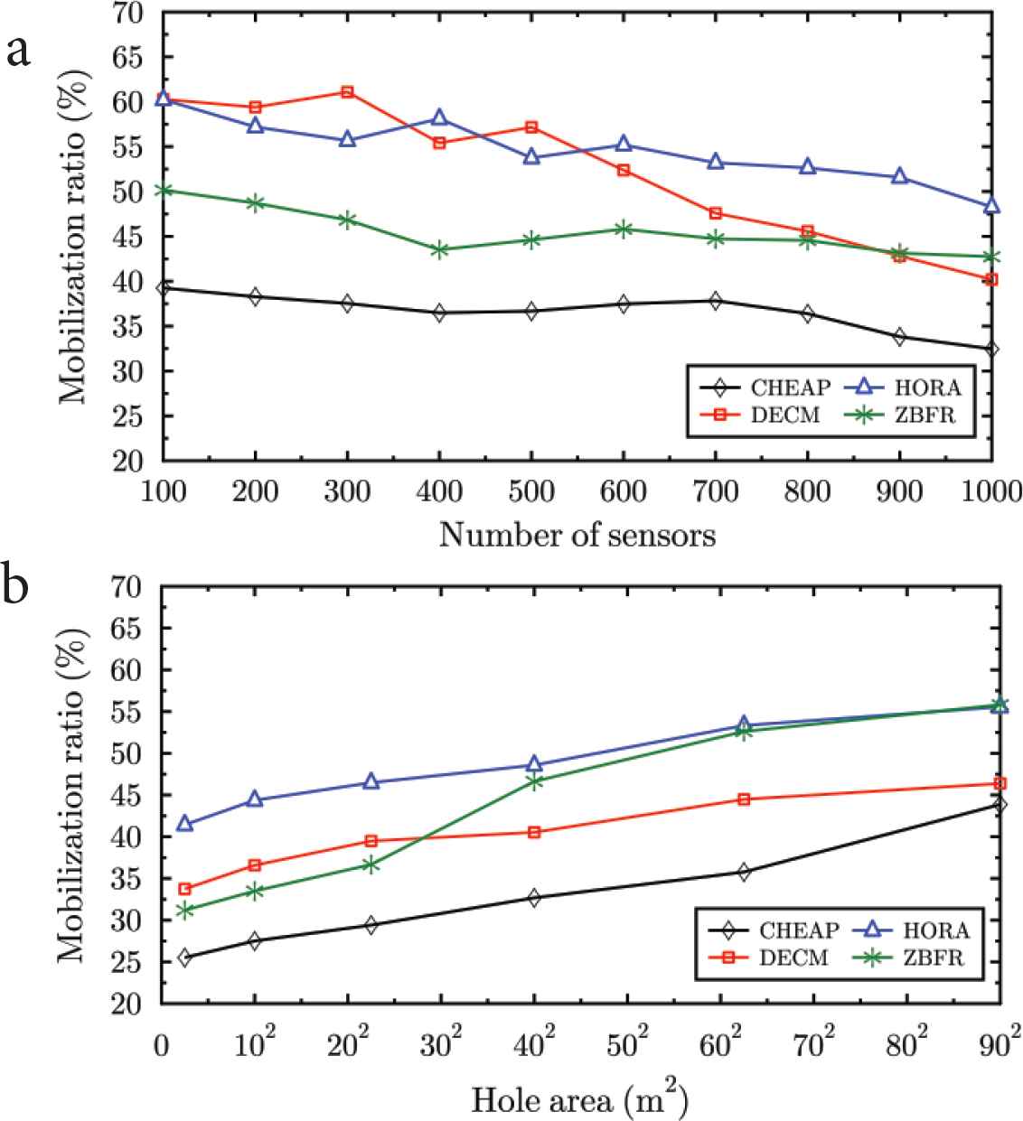
Average mobilization ratio: (a) effect of network size; (b) effect of fault scale for network size = 1000.
4.4. Average Elasticity
We carried out this experiment in order to investigate each protocol’s ability to prevent new hole formation during candidates’ relocation. After hole elimination, the simulation program searched for a hole in candidates’ coverage. This metric denotes the ratio between the number of candidates who did not make any coverage hole and the total number of candidates. The resulting ratios were averaged after all sensors died.
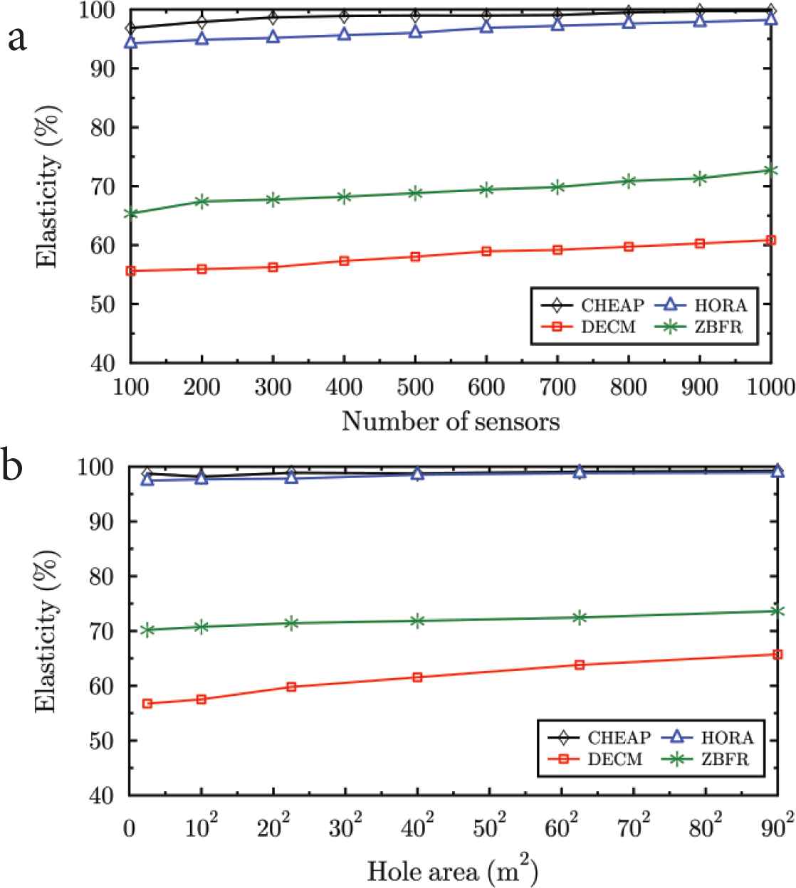
Figure 12a and 12b shows that elasticity increases according to network size and fault scale irrespective of the protocol used. These results are due to the fact that when node density is high, hole creation probability by cascaded movements is low; the same goes for the number of nodes to be relocated. DECM provides the lowest ratios (around 55%). This is because DECM can generate unnecessary node movements which reduce the Delaunay triangulation accuracy. This shortcoming is detrimental to safe area calculation and inevitably leads to new holes while candidates are moved. ZBFR yields better ratios (65–68%) because the strategy applied is mainly based on redundant nodes (back up nodes); but an insufficient number of backup nodes forces ZM to move the nearest neighbor even if a new hole is created. Thus, ZBFR actually eliminates holes through cascaded movements. The latter scheme is inefficient for holes located in the area of interest’s periphery. This issue is addressed by the linear non linear programs respectively proposed by CHEAP and HORA who both yield ratios above 90%. However, when using CHEAP, values oscillate between 96% and 99.75%. Indeed, unlike HORA, CHEAP strives to control both nodes’ ranges (motility) and mobility. These results prove the relevance of the strategy that allows each node to define a elbow room since it helps to take account of all the meaningless and risky movements.
Average elasticity: (a) effect of network size; (b) effect of fault scale for network size = 1000.
4.5. Average Migration Ratio
The goal of this experiment was to assess each protocol’s ability to minimize the travel distance required to eliminate a hole. For that purpose, after fault injection, the simulation program estimated and recorded the distance of each potential candidate to the hole’s centroid. Then, after hole elimination the simulation program calculated for each candidate, the ratio between the distance actually travelled and the distance supposed to be covered.
Note that for undetected holes the ratio is assumed to be 100% for each candidate. This experiment was ended after all sensors died.
The results depicted in Figure 13a and 13b suggest that irrespective of the protocol used, the average migration ratio decreases according to network size but increases with fault scale. These performances are due to the fact that the higher is node density the shorter is the distance to be travelled by candidates (especially, the boundary nodes) to eliminate any hole; but, for a specific network size, the larger is a hole, the longer is the distance travelled. HORA provides the worst ratios (above 90%). Indeed, in this scheme the only criterion for candidates selection is their overlapping degrees. Ignoring nodes residual energy inevitably leads to high distances travelled. When using ZBFR or DECM, the average migration ratio respectively reaches 82% and 80%. ZBFR also does not consider candidates’ residual energy but unlike HORA, the Zone Monitors relocate the nearest backup nodes (redundant nodes). DECM use a similar scheme when helping candidates find the shortest path to their safe area. Regrettably, all these performances are mitigated by the cascaded movements attached to both solutions. CHEAP outperforms the three other protocols by providing a 70% ratio on average. This performance is mainly due to the minimization scheme applied by the coordinator while selecting candidates. This strategy helps to avoid using nodes’ cascaded movements. Indeed, when using CHEAP only mutually compatible movements are allowed, this strategy prevents new hole formation and minimizes the number of movements required for coverage restoration. Furthermore, unlike DECM and HORA, CHEAP considers both nodes’ residual energy, nodes’ motility, redundant nodes’ mobility, and obstacles during the candidates selection process.
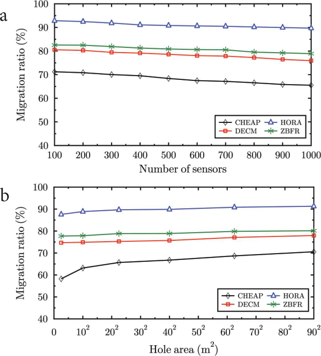
Average migration ratio: (a) effect of network size; (b) effect of fault scale for network size = 1000.
4.6. Average Elimination Ratio
In order to evaluate each protocol’s ability to restore the coverage degree we conducted an experiment where the simulation program had to calculate the area of the newly created hole just after having injected a fault. After nodes’ relocation, the resulting coverage ratio was estimated. Note that each hole which was not eliminated was assumed to have 0% coverage ratio. This experiment ended after all sensors died.
Figure 14a and 14b shows that regardless of the protocol used, the average elimination ratio increases according to network size, but decreases with fault scale.
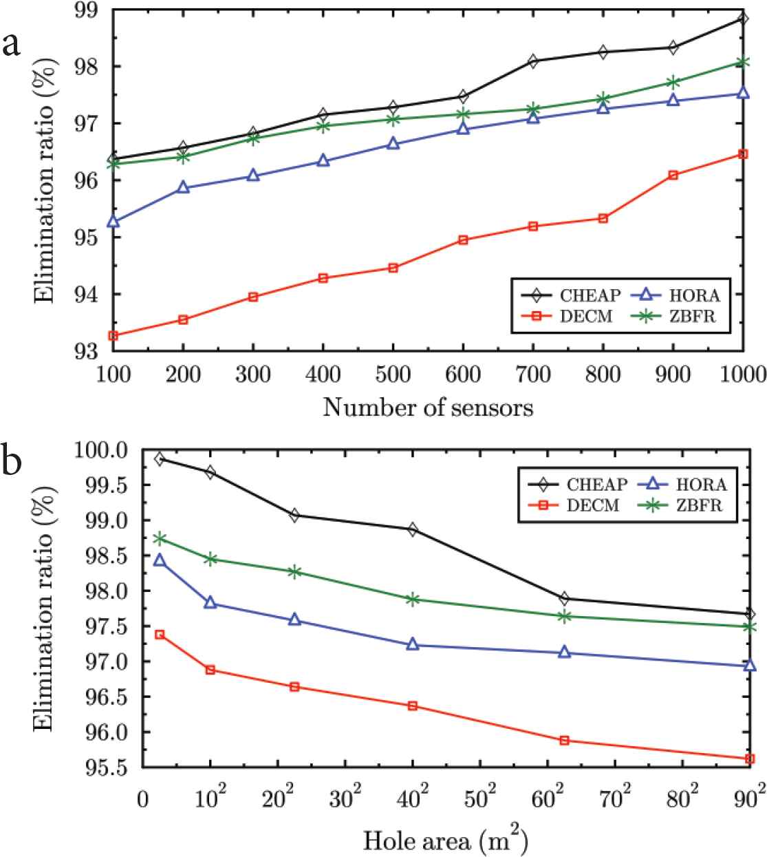
Average elimination ratio: (a) effect of network size; (b) effect of fault scale for network size = 1000.
This is because when node density is high, the number of candidates is large enough to restore the coverage. However, intuitively for the same network density, the average elimination ratio decreases when the area to be restored increases. All the evaluated protocols, provide ratios greater than 90%. DECM yields the lowest ratios (between 93% and 95.5%). This is due to the inaccuracy of Delaunay triangulation. Indeed, as discussed in Section 4.4 this scheme can lead to some errors when safe areas are calculated especially with open holes or those located in the outskirts of the area of interest. These errors are detrimental to hole full coverage. HORA and ZBFR provide better results (respectively between 95.2% and 95.6% and between 96.5% and 97%) because these schemes mainly consider redundant nodes when trying to eliminate a coverage hole; but these performances are mitigated by the fact that coverage redundancy check is a NP-complete problem [51,52] which requires approximate solutions that often lead to several false negative cases. The latter prevent efficient candidates mobility and hole full coverage. CHEAP provides the highest ratios varying between 96.5% and 98%. This is due to the fact that during the hole elimination process, when making decisions coordinator uses candidates’ maximum range while targeting primarily the centroid. The latter position often provides the highest coverage ratio when using node’s maximum range.
4.7. Energy Efficiency and Network Lifetime
In order to estimate the amount of energy depleted during hole detection and elimination processes, we used the same experimental setup as described in the previous sections. Since we mainly aimed at investigating each protocol’s ability to minimize energy losses, we injected only faults that displaced nodes. We conducted this experiment respectively until a node died [First Node Dies (FND)] and until all nodes died [Last Node Dies (LND)].
Figure 15a and 15b then 16a and 16b show that irrespective of the protocol used and the lifetime definition (FND or LND), the energy oriented network lifetime decreases while network size and fault scale grow. These results are due to the fact that energy losses are mainly due to communication activities. The latter increase according to nodes’ degree (number of neighbors). By contrast, large scale disasters (especially when several nodes become isolated) tend to decrease nodes’ average degree and reduce therefore their energy consumption. However, since faults are essentially local, they have a relatively small impact on the network’s lifetime. CHEAP obtains the best results. They are actually due to its performances in terms of message complexity and average migration or mobilization ratio, as discussed in previous sections. By contrast DECM, ZBFR, and HORA use more energy consuming strategies such as cascaded movements. Indeed, ZBFR uses heart-beat signalization scheme for hole detection while DECM leads to unnecessary node movements due to Delaunay triangulation inaccuracy (see Section 4.4). HORA does not consider residual energy to select candidates for coverage recovery. The latter strategy is particularly energy inefficient.
Network lifetime (until First Node Dies): (a) effect of network size; (b) effect of fault scale for network size = 1000.
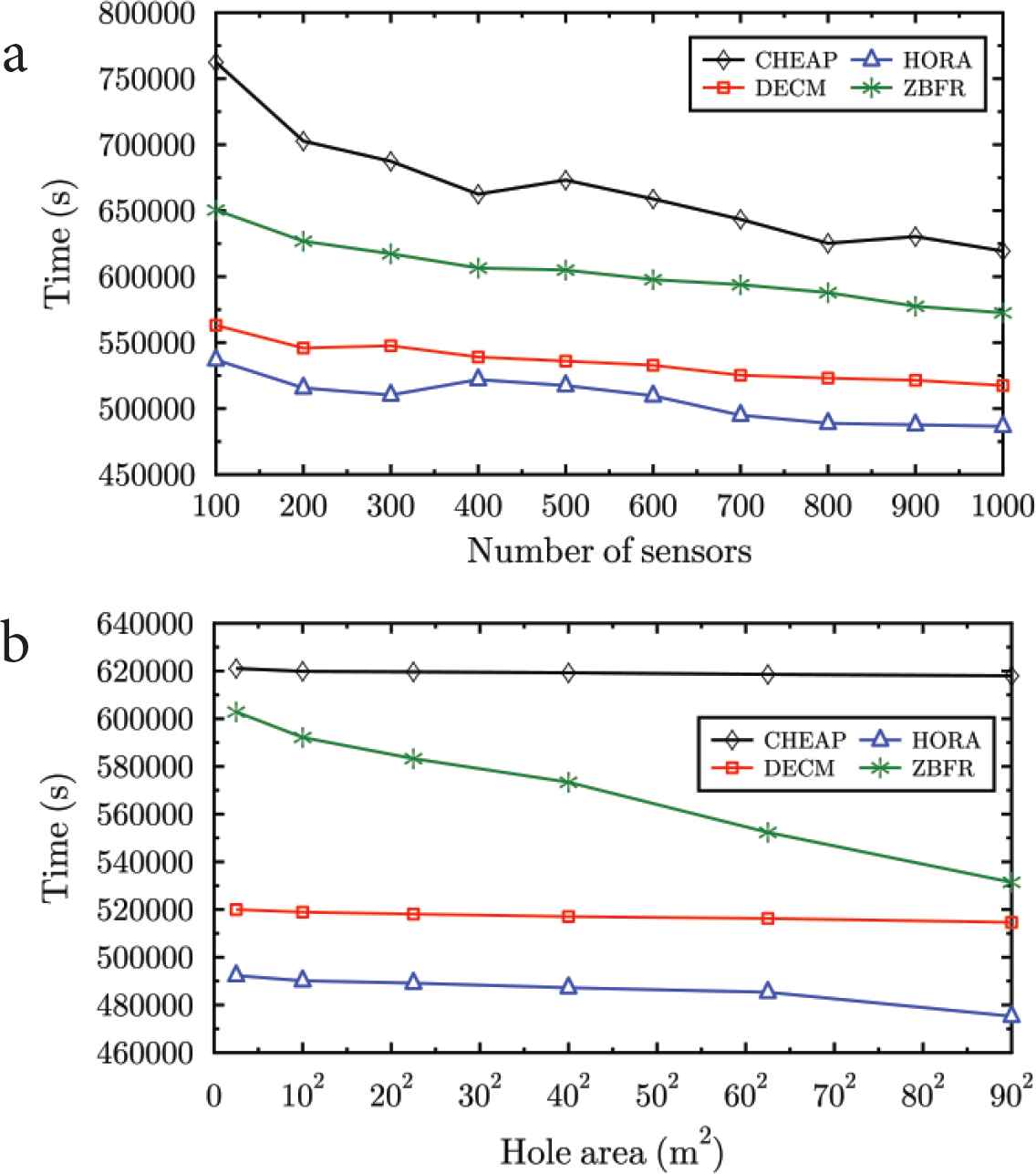
Network lifetime (until Last Node Dies): (a) effect of network size; (b) effect of fault scale for network size = 1000.
4.8. Coverage Resilience Index
In order to evaluate each protocol’s ability to maximize network resilience denoted by φ, we propose to aggregate the metrics discussed above using a weighted geometric mean as expressed by Equation (34). Let τm, ls, τg, τe, and ε respectively be the average mobilization ratio, the average elasticity, the migration ratio, the average elimination ratio, and the average energy consumption ratio.
By definition, a candidate’s energy consumption ratio is the amount of energy lost during the entire coverage maintenance process divided by its residual energy at the time of fault injection.
Figure 17a and 17b shows that regardless the protocol used, resilience increases according network size, but decreases as fault scale grows. These results are due to the fact that high node density intuitively fosters coverage recovery speed and ratio. Since this resilience index is a composite metric, any performance depends on the results discussed in previous section. CHEAP provides a coverage resilience index between 70% and 74.2%. In other words, our contribution enables network to efficiently maintain coverage in 70–74.2% of all cases; while the three other protocols’ results oscillate between 45% and 57%. These results prove that the coordination and location-allocation-based strategy combined with nodes’ range control is more relevant than any iterative movements-based scheme to eliminate coverage holes.
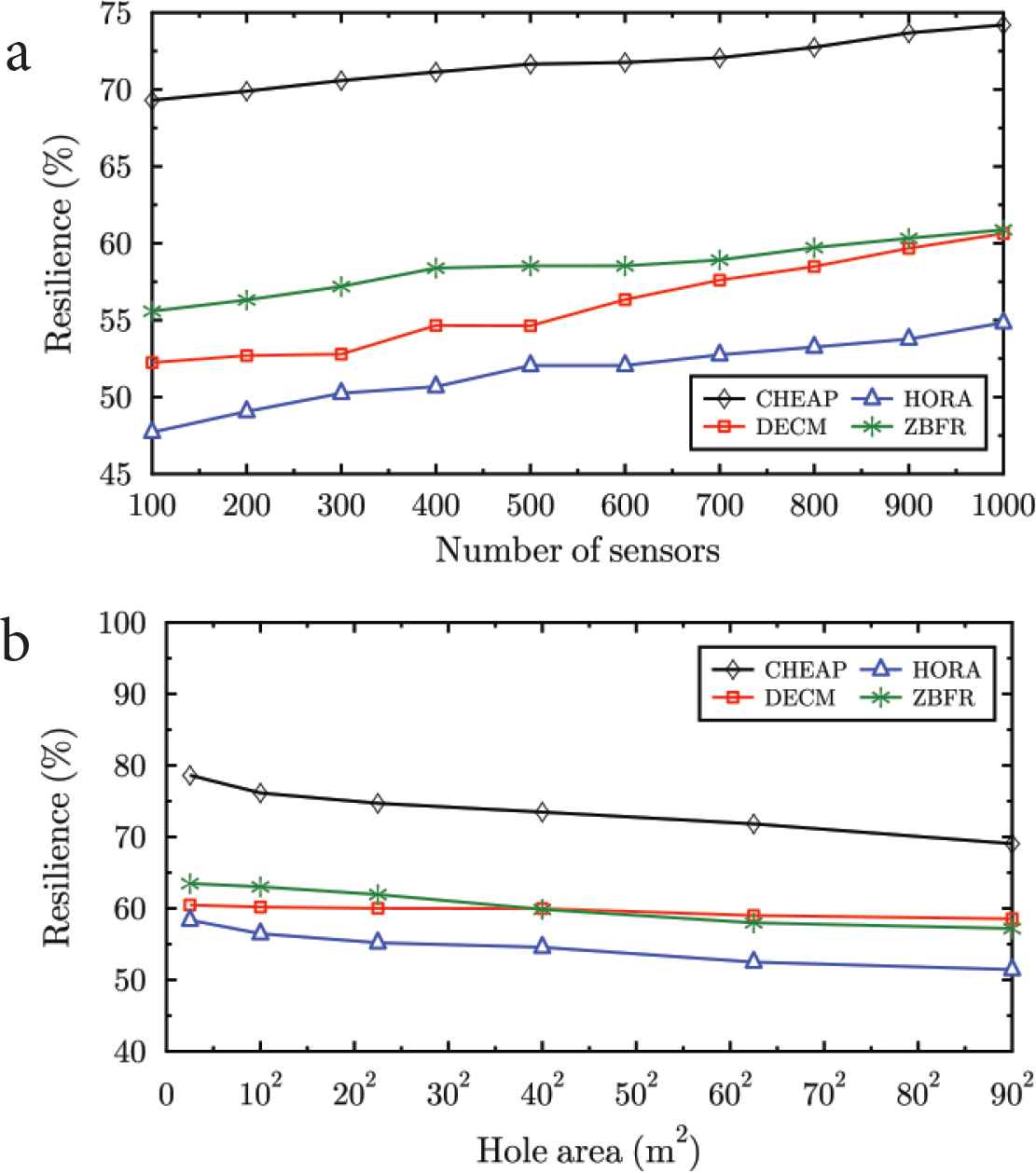
Resilience: (a) effect of network size; (b) effect of fault scale for network size = 1000.
5. CONCLUSION
In this paper we addressed the area coverage restoration problem in self-organized mobile WSNs with the objective of maximizing the network’s resilience. We proposed a localized solution referred to as CHEAP that uses first, a geometric approach based on nodes’ sensing disks crossings to effectively detect any type of holes; then a tabu search based heuristic that combines nodes’ redundancy, motility and mobility-based strategies to restore the lost coverage. Simulation results have confirmed that regardless of the type of hole, CHEAP outperforms several major previous schemes. The coverage resilience index metric we proposed, explicitly revealed that the location-allocation-based scheme we applied helps to effectively minimize risks of new hole formation, average distance travelled, nodes’ movements, overlapped areas, and total power consumption; while maximizing coverage ratio.
In future work, we plan to extend this solution to three-dimensional environments.
CONFLICTS OF INTEREST
The authors declare that they have no known competing financial interests or personal relationships that could have appeared to influence the work reported in this paper.
Footnotes
REFERENCES
Cite this article
TY  - JOUR
AU  - Gokou Hervé Fabrice Diédié
AU  - Boko Aka
AU  - Michel Babri
PY  - 2021
DA  - 2021/01/18
TI  - CHEAP: An Efficient Localized Area Coverage Maintenance Protocol for Wireless Sensor Networks
JO  - International Journal of Networked and Distributed Computing
SP  - 33
EP  - 51
VL  - 9
IS  - 1
SN  - 2211-7946
UR  - https://doi.org/10.2991/ijndc.k.201218.001
DO  - 10.2991/ijndc.k.201218.001
ID  - Diédié2021
ER  -