
Modified Ant Colony Optimization Algorithm for Multiple-vehicle Traveling Salesman Problems
- DOI
- 10.2991/ijndc.2018.7.1.4How to use a DOI?
- Keywords
- Multiple-vehicle traveling salesmen problem; ant system; local search; simulated annealing; 2-opt; 3-opt
- Abstract
In this work, we extended the original Traveling Salesman Problem (TSP) to cover not only the case of multiple vehicles but also to constrain the minimum and maximum numbers of cities each vehicle can visit. Our algorithm is a modified Ant Colony Optimization (ACO) algorithm which has the ability to avoid local optima; our algorithm can be applied to transportation problem that covers either a single vehicle or multiple vehicles. To the original ACO, we added a new reproduction method, a new pheromone updating strategy, and four improved local search strategies. We tested our algorithm on several standard datasets in the TSP library. Its single-vehicle performance was compared to that of ant system (AS) and elitist ant system (EAS) algorithms. Its multiple-vehicle performance was evaluated against that of ant colony system variants reported in the literature. The experiments show that our proposed ACO’s single-vehicle performance was superior to that of AS and EAS on every tested dataset and its multiple-vehicle performance was excellent.
- Copyright
- © 2018 The Authors. Published by Atlantis Press SARL.
- Open Access
- This is an open access article under the CC BY-NC license (http://creativecommons.org/licences/by-nc/4.0/).
1. INTRODUCTION
Currently, business and industry sectors are giving increasingly higher priority to transportation and distribution of goods because the oil price which determines a transportation cost is ever increasing. Transportation and distribution of goods are the most expensive logistics activities; therefore, businesses are keen to increase the efficiency and reduce the cost of transportation—especially, they have brought in new information technology to help reduce the cost of transportation, i.e. reduce the amount of fuel used for transportation, reduce the maintenance cost, etc. Generally, transportation cost varies with the distance; an efficient routing scheme can reduce the cost of transportation substantially, which in turn, reduces the cost of goods. Meta-heuristic algorithms have been used successfully by manufacturers to reduce transport costs and enhance the business. Algorithms of this type generally find a satisfactory solution to problems, which are inherently nondeterministic polynomial-time hard (NP-hard), in an acceptably short time [1,2]. Meta-heuristic algorithms have also been applied to Traveling Salesman Problem (TSP), a classic NP-hard problem that tries to find the shortest tour that a salesman can take to visit all of his customer sites in a single tour, with starting and end points at the same city. However, when the search space is large and there are numerous cities or nodes which must be touched, the problems cannot be modeled as the original TSP with only one salesman. Real-world applications of such problems are print scheduling, workforce planning, production planning, transportation planning, etc. [3]. To address this problem, Multiple-Vehicle Traveling Salesman Problems (MTSP) have been developed under the constraints that each city is to be visited only once by only one salesman and the starting and end points are the same city; the objective is to minimize the total distance of all of the tours. Possible variations of MTSP include: (i) single depot or multiple depots—for the case of a single depot, the origin and destination for every salesman is the same, while, for the case of multiple depots, the origins and destinations for any salesman can be any depot; (ii) the number of salesmen can be any number, i.e. user-defined; (iii) fixed charges—with multiple salesmen, there may be a certain fixed cost for a particular salesman responsible for a particular tour plus the cost of the tour; (iv) time window—each city must be visited within a time window that may be different for different problems, such as for a school bus routing problem or for an airline scheduling problem; (v) other constraints, such as the number of cities that each salesman can visit or the maximum or minimum distances that a salesman can travel [4,5].
Several researchers have discussed the MTSP. For example, Xu et al. [6] described a Two Phase Heuristic Algorithm (TPHA) for MTSP. They achieved a balanced workload and minimized the total distance, that a salesman takes, by using a K-means algorithm in the first phase to group all cities into several subsets depending on their locations and by using a genetic algorithm (GA) in the second phase to assess the route for each subset. A roulette wheel selection method and an elitist strategy are combined to form a new selection operator for the GA. In addition, they introduced a mobile application that incorporated this TPHA for travelers based on a Baidu electronic map. The TPHA was found to be better at finding a solution to MTSP than a GA-based tour planning algorithm. In another study, Zhou et al. [7] described Partheno Genetic Algorithm (PGA) and Improved Partheno Genetic Algorithm (IPGA) for solving MTSP, with multiple depots where the starting and end points were the same depot and each salesman had to visit a required minimum number of cities. PGA uses a roulette wheel selection method and an elitist selection method with four types of mutation, i.e. FlipInsert, SwapInsert, LSlideInsert and RSlideInsert. On the other hand, IPGA uses the same selection methods as those of PGA but added mutation probability. They claimed improved performance compared to those of a modified particle swarm optimization algorithm and an invasive weed optimization algorithm. Although there are many papers devoted to MTSP, but they cannot be used as a benchmark because they did not state clearly and unequivocally the conditions and constraints of the MTSP that they solved. However, Necula et al. [8] carefully determined which of the several ant colony algorithms produced the best balanced workload for each salesman and the best total tour cost reduction. They investigated five different ant colony system algorithms for MTSP: Km-Ant Colony System (ACS) that decomposed MTSP by using K-means; g-ACS that combined ACS with global-solution pheromone update; s-ACS that combined ACS with sub-tour pheromone update; gb-ACS that combined ACS with global-solution pheromone update and bounded tours; and sb-ACS that combined ACS with sub-tour pheromone update and bounded tours. The results showed that a Km-ACS was a good benchmark for a single-depot MTSP. In addition, Wang et al. [9] used a novel memetic algorithm incorporating a sequential variable neighborhood descent (seq_VND) method. At each iteration, the best individual among the reproduced offspring is improved by the seq_VND. The seq_VND ordered the neighborhoods in a sequence and visited one-by-one until a local minimum is reached. This algorithm was evaluated on large-scale benchmark problems (up to 1173 cities). It was also evaluated against six other algorithms in terms of precision, robustness and convergence speed. The results showed that it was superior to all of the other algorithms. Kencana et al. [10] solved the MTSP with an ant system (AS) algorithm. They found the shortest tour for five to ten salesmen visiting up to 30 cities. Their study produced similar results to other studies, but the minimum total tour distance and completion time were longer. Moreover, it did not guarantee that a higher number of salesmen would reduce the length of the tour. Finally, Soylu [11] used a General Variable Neighborhood Search (GVNS) approach for MTSP; he was motivated to use it for solving the traffic signalization network in Kayseri Province, Turkey. The network had 170 nodes and six sub-networks. In this problem, the sub-network lengths were not balanced and the network was so large that a suitable alternative could not be easily found. GVNS was able to obtain a significant improvement in terms of maximum tour length and range.
The MTSP mentioned above used various types of constraints found from real-life applications such as a single depot or multiple depots, a small or large number of nodes (cities to be visited). In our study, we aimed to develop an algorithm for solving both a TSP under the constraints of a single depot and only one vehicle that would deliver all of the goods to all customers, as well as an MTSP under the constraints of a single depot and multiple vehicles that would minimize the total length of the tour while keeping the workloads of the salesmen balanced. Moreover, it should allow for a pre-determined number of multiple vehicles for each tour, as well as pre-determined minimum and maximum numbers of cities in each sub-route that each vehicle would visit. However, there would be no constraints on delivery time or vehicle capacity. In this paper, we improved tour reproduction, pheromone updating, and local search strategies. Four strategies—simulated annealing (SA), simulated annealing with similarity measure (SA_Sim), 2-opt and 3-opt—were used to improve local search capability. We evaluated performance on several instances in the TSP Library (TSPLIB) dataset. For the single-vehicle TSP, we compared results with those achieved by AS algorithm and elitist ant system (EAS). Our multiple-vehicle performance was evaluated against that of five variants of the ACS reported in the literature.
The remainder of this paper is organized as follows: Section 2 describes in detail the basic concepts and steps of the AS algorithm. Section 3 presents our proposed method. Section 4 reports the performance evaluation results of the proposed method. Finally, Section 5 is the conclusion.
2. RELATED ALGORITHM
2.1. Basic AS Algorithm
In the last two decades, many researchers have attempted to combine ideas from the bioscience domain with those in computational mathematics. Specifically, they have tried to solve some mathematical problems by integrating animal behaviors into certain computational techniques. Ant system algorithm is based on a self-organization mechanism of social insects [12]. This algorithm mimics the behavior of ants trying to search for the shortest tour from their nest to food sources. On the path that they traverse, they leave traces of pheromones. The pheromone density depends on the distance between the food source and the nest as well as the quality of the food source. Ants tend to follow the tour with the maximum pheromone density laid down by previous ants. This idea was adapted to solve the standard TSP problem [13–15].
2.2. Steps of AS Algorithm
Basically, an AS algorithm has two main parts: tour construction and pheromone update. At the beginning of the tour construction, m ants are randomly placed in one of n cities. The rule for choosing a city that each of the ants will visit in its next move is in the form of a probability that the kth ant, currently at the ith city, will move to the jth city, as shown in Equations (1) and (2).
After all of the ants have constructed their initial tour, the pheromone updating process begins. As expressed in Equation (3), the pheromone updating process consists of two activities: (i) the pheromone is laid down by ants while traversing the paths, and (ii) the amount of pheromone on all paths is decreased with time by a constant factor called pheromone evaporation rate.
3. PROPOSED ALGORITHM
We developed our algorithm to remedy the following deficiencies of the AS algorithm: (i) insufficient population diversity, since the path that has the highest pheromone density is always taken; (ii) premature convergence and becoming trapped in local optima; and (iii) the quality of the solutions degrade as the number of cities increases. A key contribution is the addition of a new tour reproduction method. This new method allows a stronger ant to reproduce two tours whereas a weaker one reproduces only one, so the stronger ant will contribute more to finding better solution.
Another contribution is the introduction of a weight of each tour; with a shorter tour having a higher weight. The last contribution improves local search by randomly choosing one of these four strategies: simulated annealing (SA), simulated annealing with similarity measure (SA_Sim), 2-opt and 3-opt. Using these fours strategies increases the chance that a solution will escape from a local optimum. The flowchart of the proposed algorithm is displayed in Figure 1.
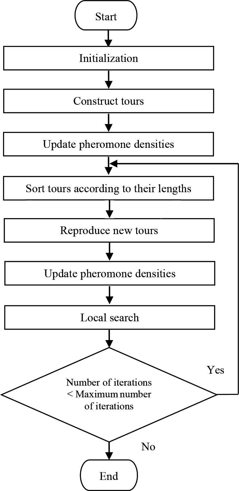
Flowchart of the proposed algorithm
In detail, the steps are:
Step 1: Initialize the total number of tours (m), the total number of cities, the initial pheromone value (τ0), the pheromone evaporation rate (ρ), α and β that control the relative importance of the pheromone trail and the visibility, the total number of vehicles (V), the minimum number of cities that each vehicle will visit, the maximum number of cities that each vehicle will visit, and the maximum number of iterations.
Step 2: Randomly generate each tour. The distance between the ith and the jth cities of each sub-route in a tour is di,j, di,j = [(xi − xj)2 + (yi − yj)2]1/2. The length of the sub-route for vehicle s is Ls [Equation (5)].
where d0,1 is the distance between the depot and the first city in the sub-route;where V is the total number of vehicles.Step 3: Update the amount of pheromone on every path. The updated amount of pheromone on each path is [Equation (7)]:
whereWhere Lshortest is the shortest tour of a particular iteration and Llongest is the longest tour of that iteration.Step 4: Sort the tours according to their length from the shortest to the longest.
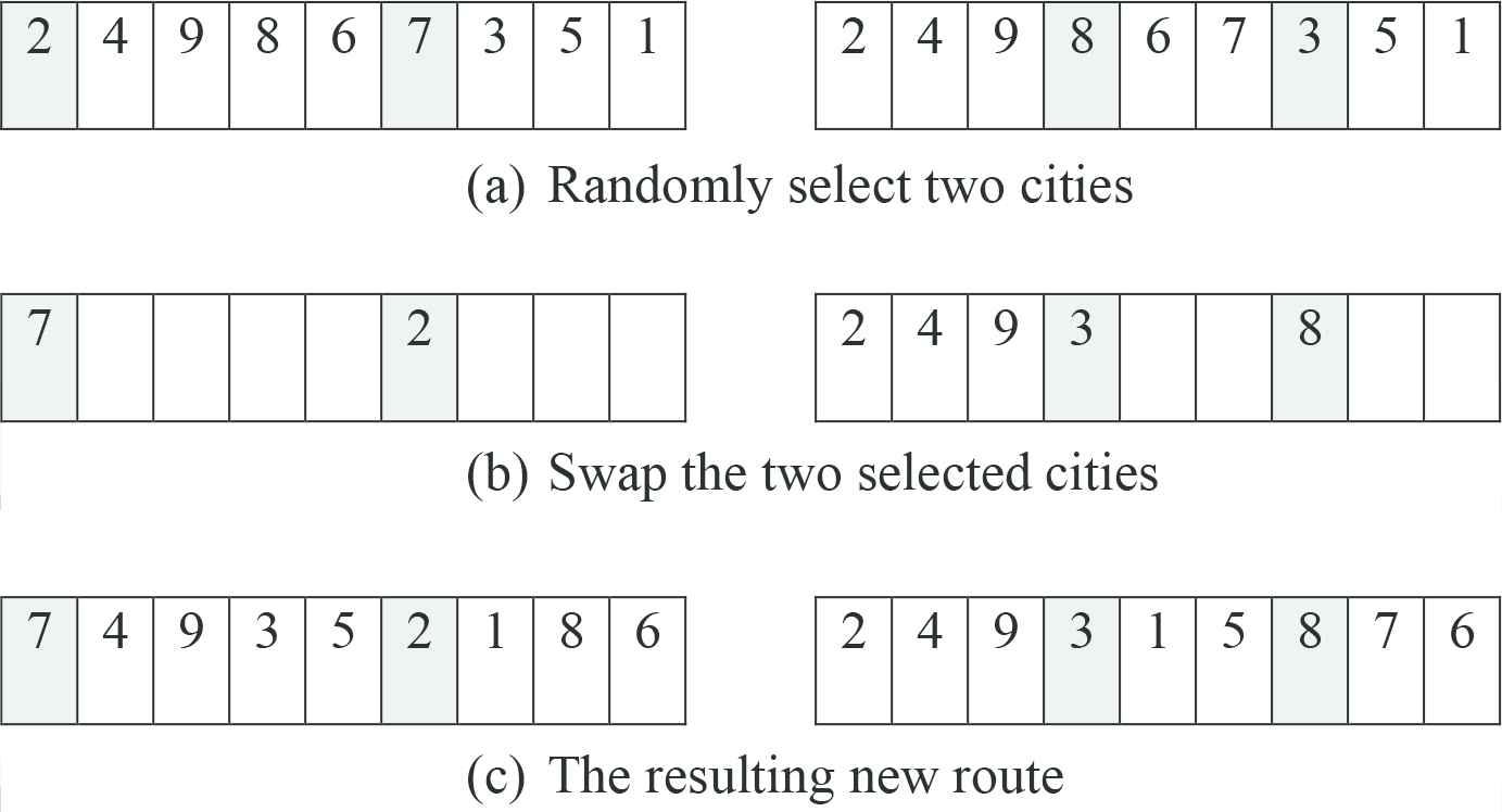
Step 5: Divide the tours into two groups: the top 20% and the bottom 80%. The tours in each group are cloned differently. Tours in the top 20% group generate two new tours whereas those in the bottom 80% generate only one new tour. Each new tour is constructed by randomly selecting two cities in the original tour and swapping them. The rest of the cities that have not been swapped are arranged as follows. In the case that the first city was randomly selected for swapping, the cities in the slots between and after the swapped cities are changed according to the probability for selecting the next city in Equation (1). However, if the first city of the selected tour was not selected for swapping, the city or cities located in the slot(s) before the first of the swapped cities remain the same (see Figure 2), while the city or cities in the slot(s) between the swapped cities and those following them are changed according to the probability in Equation (1). Figure 2 shows two examples of this procedure. In the first (left-hand side) example, “2” and “7” were randomly selected. After swapping, “7” became the first city of the tour. The possible cities to traverse to next are “1”, “3”, “4”, “5”, “6”, “8”, or “9”. The probability for selecting these cities as the next city are (P71 = 10), (P73 = 22), (P74 = 25), (P75 = 21), (P76 = 14), (P78 = 18), and (P79 = 22). Therefore, the next path will be toward city “4” that has the highest probability. If a city has already been visited, it will be removed from the list. The path to the next city is determined in the same way until the list of next possible cities is empty.
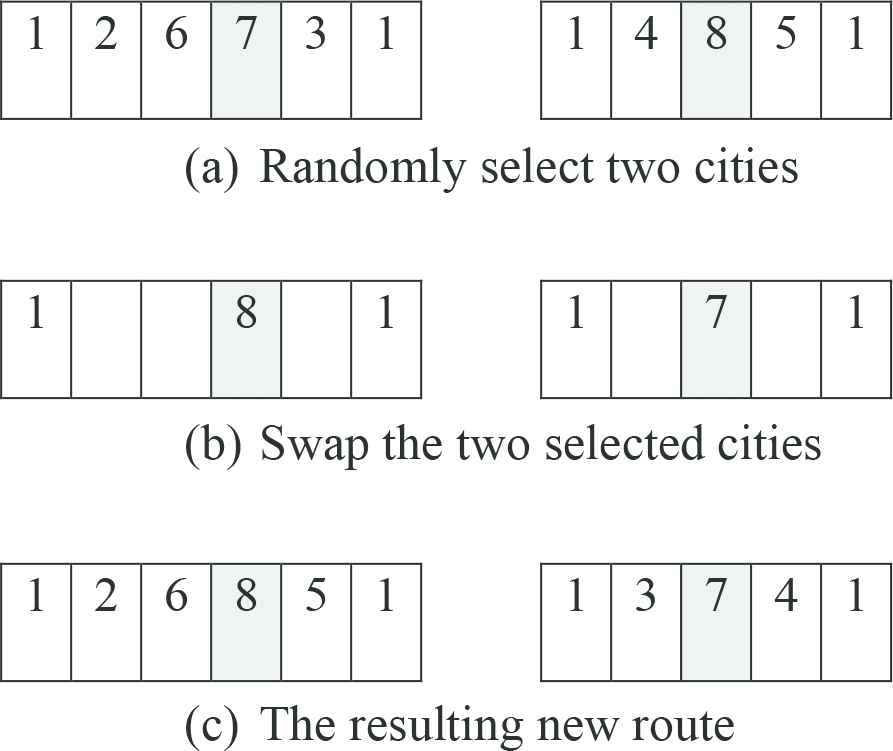
The description above is for the case of randomly selecting and swapping two cities in the same sub-route. On the other hand, Figure 3 illustrates the procedure for reproducing a new tour from two different sub-routes. This procedure further improves the diversity of the original tour. To begin with, the two sub-routes are randomly selected from all possible sub-routes in the original tour. Assuming “1” is the depot. After “7” and “8” in the two different sub-routes have been randomly selected and swapped, the city or cities located in the slot(s) before the first swapped city remain the same (see Figure 3), while the city or cities in the slot(s) between the swapped cities and those following them are changed following Equation (1). In the left-hand side sub-route in Figure 3 which is the first sub-route that was randomly selected, “8” is the city that has been swapped, hence similar to the procedure for swapping cities within a sub-route above, “2” and “6” take the same position that they have in the original sub-route; the possible cities to traverse to next in this sub-route are then “3”, “4”, or “5”. The probabilities are P83 = 20, P84 = 26, and P85 = 30. Therefore, the next path will be toward city “5”. Then, in the right-hand side sub-route which is the second sub-route that was randomly selected, the left-most unassigned slot is assigned city “3” because the probability of taking these paths are P53 = 25 and P54 = 20, and the last unassigned slot receives city “4”.
Step 6: Use Equation (7) to update the amount of pheromone on all the paths with the new tours created in Step 5. Combine the lists of initial and new tours, and then sort based on the tour length from the shortest to the longest. The top m ranked tours are selected for the next step. The shortest tour, Tour_best, is recorded.
Step 7: Improve the quality of the tours by using one of the four local search strategies. To start with, each of the m tours is randomly assigned to one of the four lists: LSA, LSA_Sim, L2-opt, and L3-opt. Each list corresponds to a particular strategy. In the first iteration (t = 1), all strategies have the same probability of being chosen (PSA(t) = PSA_Sim(t) = P2-opt(t) = P3-opt(t) = 0.25). In the subsequent iterations, however, the probability of being chosen for each strategy is updated to reflect the performance in improving the quality of the tour of that strategy. The method used in this updating process follows Qin et al. [16].
The first strategy uses the SA algorithm to improve the tour quality in LSA as follows:
- •
Firstly, randomly select one of the three heuristics in SA (insert_mutation, inverse_mutation, and exchange_mutation) and apply it to the tour thus creating a new tour.
- •
Compute the length of the new tour.
- •
Compute the change in length between the new tour and the original tour [Equation (9)]:
where Lnew is the length of the new tour; and Lcurrent is the length of the current tour. If E ≤ 0, replace the current tour with the new tour. However, if E ≥ 0, compute the probability eE/T and compare it with a randomly generated real number in [0, 1]. If the generated random number is less than or equal to the probability, replace the current tour with the new tour, else keep the current tour. The temperature, T, in each SA iteration is calculated by Equation (10):where tstart is the initial temperature; tend is the final temperature; iter is the current iteration; and iter_max is the maximum number of iterations specified beforehand. - •
Repeat the above procedure until the maximum number of iterations is reached.
- •
The best tour achieved by this strategy is grouped with the original tours from Step 6 and other new tours achieved by the other local search strategies.
Two examples of reproduction of a new tour from a sub-route
Example of reproduction of a new tour from two different sub-routes
The second strategy uses the SA_Sim algorithm to improve the quality of each tour in LSA_Sim.
- •
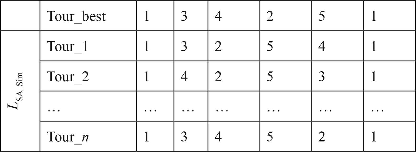
Initially, the similarities between Tour_best and all tours in LSA_Sim are determined. Pair up Tour_best with all of the tours in LSA_Sim as shown in Figure 4 and determine their similarity values. From the example in Figure 4, the similarity value between Tour_best and Tour_1 is determined as follows: the first path of both tours is the same (city 1 → city 3) so the similarity value for this path is 1. Next, the second path of Tour_best is 3 → 4, but no paths of Tour _1 is 3 → 4, so the similarity value for this path is 0. On the other hand, the fourth path of Tour_best is 2 → 5 which is similar to the third path of Tour_1, so the similarity value for this path is also 1. It can be observed that all of the other paths in Tour_best and Tour_1 are not similar, so the total similarity value between Tour_best and Tour_1 is the sum of the similarity values of all of the paths in both tours which is 2 in this example.
- •
The obtained similarity values between Tour_best and all of the tours in LSA_Sim are then used to calculate the probability of taking SA.
where PSAi is the probability of taking SA for the tour i. Similarityi is the similarity value between Tour_best and the tour i in LSA_Sim; dim is the total number of paths in the tour. - •
For each tour in the LSA_Sim, if a random number in [0, 1] is less than or equal to the probability of taking SA, follow the steps of the SA algorithm above, else keep the current tour.
- •
Group the best tour achieved by this strategy with the original tours from Step 6 and other new tours achieved by the other local search strategies.
The third strategy uses the 2-Opt algorithm which randomly selects two sub-routes and swaps some cities between them [17,18]. The steps of the algorithm are demonstrated in the example below.
- •
Figure 5 shows an example of a tour consisting of four sub-routes.
- •
A sub-route (the second sub-route in Figure 6a labelled sub-route 1) and a path from city 10 → 12 in this sub-route are randomly selected (paths that begin or end at city 1, the depot, are discarded if randomly selected) then another sub-route (labelled sub-route 2) is randomly selected. This sub-route 2 (in Figure 6a) must be randomly selected from only sub-routes that come after sub-route 1 in the sequence.
- •
The randomly selected path, 10 →12, in sub-route 1 is matched to each path in sub-route 2, except 1 →2 and 8 →1, because city 1 is the depot.
- •
Swap the destination city in the selected path in sub-route 1 (i.e., 12) with the origin city in each of the matched paths in sub-route 2. For example, for the first matched pair, swap 12 ↔ 2; for the second match pair, swap 12 ↔ 4; for the last matched pair, swap 12 ↔ 7. Then, the other cities located between the swapped cities are rearranged in reverse order. This procedure produces several new tours; in our example, three new tours, as shown in Figure 6a–c, are created.
- •
Compute the lengths of the tours with these new sub-routes and compare them with the length of the original tour.
- •
Group the best tour achieved by this strategy with the original tours from Step 6 and other new tours achieved by the other local search strategies.
Example of a tour list in SA_Sim
The fourth strategy uses 3-Opt algorithm which randomly selects three sub-routes and swaps some cities among them [18]. The steps of this algorithm are demonstrated by using an example of tour comprising four sub-routes in Figure 7.
- •
A sub-route (the second sub-route in Figure 8a labelled sub-route 1) and a path from city 8 →14 in this sub-route are randomly selected (paths that begin or end at city 1, the depot, are discarded if randomly selected). Then another sub-route (labelled sub-route 2) and a path 7 →9 in this sub-route are randomly selected. This sub-route 2 must be randomly selected from among only the sub-routes that come after sub-route 1 in the sequence. Next, another sub-route (called sub-route 3) is randomly selected. Sub-route 3 (in Figure 8a) must be randomly selected from among only the sub-routes that come after sub-route 2 in the sequence.
- •
The randomly selected path, 8 →14, in sub-route 1 and the path, 7 →9, in sub-route 2 are matched to each path in sub-route 3, except 1 →6 and 12 →1 because city 1 is the depot.
- •
For the matched paths between the path 8 →14 in sub-route 1 and the path 7 →9 in sub-route 2 to the path 6 →4 in sub-route 3, the following procedure is used: the destination city of the selected path in sub-route 1 (i.e., 14) replaces the destination city of the selected path in sub-route 3 (i.e., 4); the destination city of the selected path in sub-route 3 (i.e., 4) replaces the destination city of the selected path in sub-route 2 (i.e., 9); and the destination city of the selected path in sub-route 2 (i.e., city 9) replaces the destination city of the selected path in sub-route 1 (i.e., city 14). All of the other cities remain at the same positions as shown in Figure 8a. The same procedure is used on the matched paths between the path 8 →14 in sub-route 1 and the path 7 →9 in sub-route 2 to the path 4 →12 in sub-route 3.
- •
Compute the lengths of the new tours (two new tours in our example above) then compare the new tour lengths to the original tour length. The best tour achieved by this strategy is grouped with the original tours from Step 6 and other new tours achieved by the other local search strategies.

Example of a tour used to illustrate 2-opt algorithm
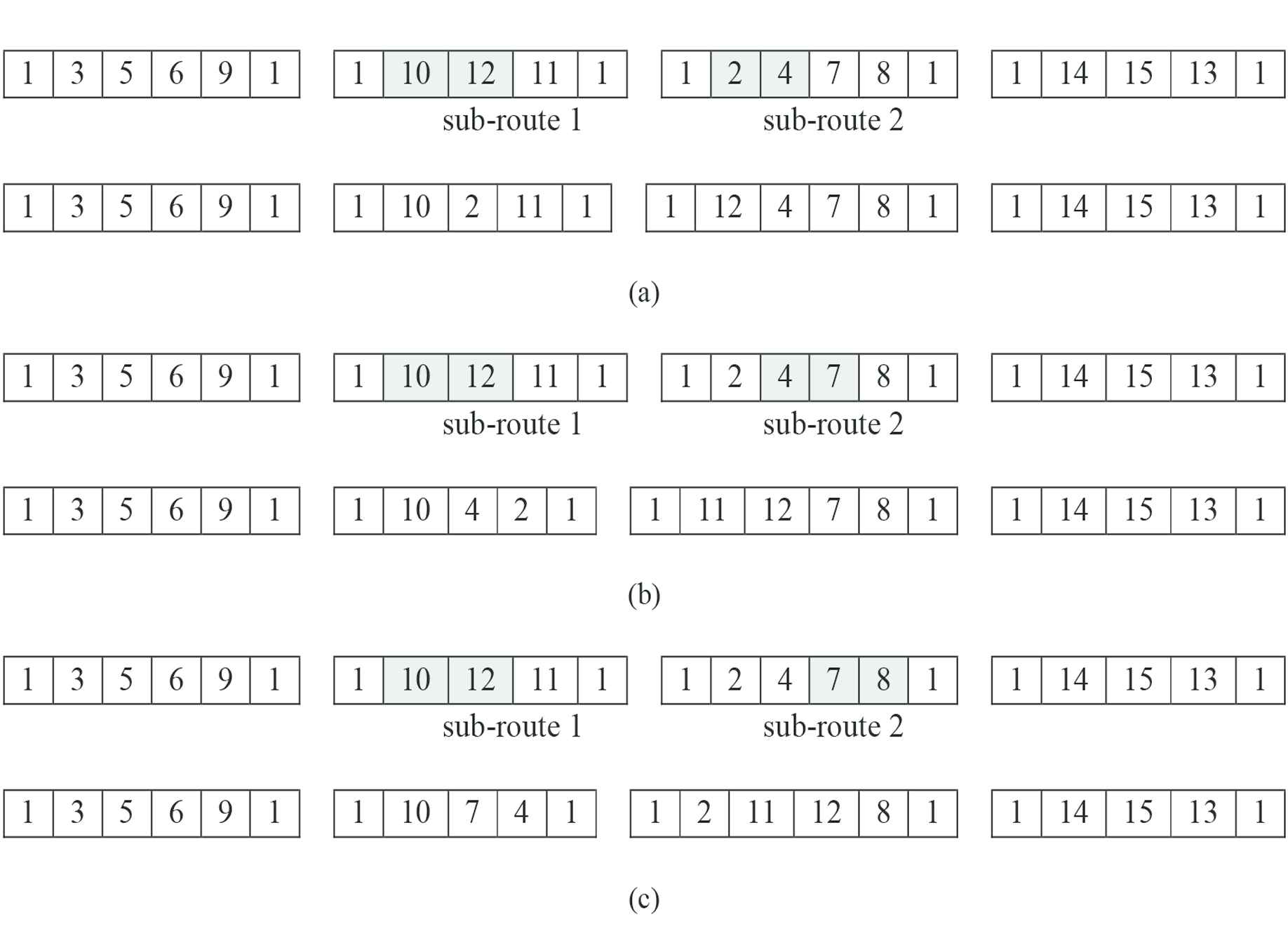
Illustration of 2-opt algorithm

Example of a tour used to illustrate 3-opt algorithm
The original tours (from Step 6) and the new tours generated by all of the strategies mentioned above are sorted based on the tour length from the shortest to the longest. Then, the top m ranked tours are selected and put into the same group. These selected tours are labelled “successful” while the tours that are not selected are labelled “unsuccessful”. These “unsuccessful” tours are put into another group.
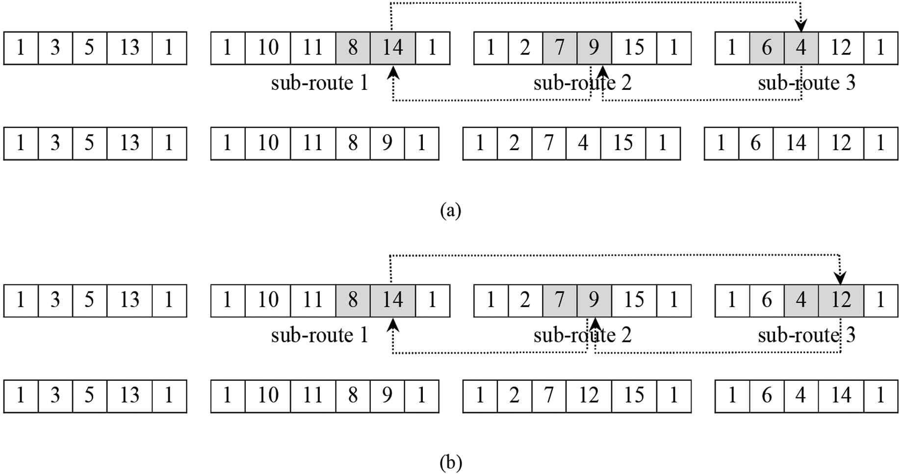
Illustration of 3-opt algorithm
Then, the success rate of each strategy (from the four local search strategies) is computed as in Equation (12):
Step 8: Record the best tour as well as its tour length.
Step 9: Repeat Steps 4–8 until the maximum number of iterations is reached.
4. EXPERIMENTAL RESULTS AND DISCUSSION
We measured the performance of our algorithm as well as other major algorithms on TSP data from TSPLIB [19]. For the single-vehicle TSP, the results of our algorithm were compared with those achieved by the ant system algorithm and EAS. For the single-depot MTSP, the performance of the proposed algorithm was evaluated against five variants of the ACS [8]. The algorithm was terminated after 10,000 iterations and each algorithm run 10 times. Each run started with a different initial population and stopped when the maximum number of iterations was reached.
Table 1 shows the experimental results on the single-vehicle TSP. The results shown in Table 1 are the shortest tour length achieved by each algorithm and the number of iterations to reach the best solution, follow in brackets. It can be clearly seen that our algorithm achieved near-optimum solutions on all tested datasets. In contrast, AS and EAS algorithms did not return good results. They fall behind our algorithm on all datasets. Among them, AS algorithm converged closer to the global minimum for eil51, eil76, and eil101 while EAS algorithm converged closer to the global minimum for att48, st70, pr76, kroC100, rd100, lin105, ch130, ch150, rat195, and kroB200. AS and EAS algorithms achieved similar results for berlin52, rat99, kroA100, and kroA200. Even though our algorithm required a significantly larger number of iterations to reach the best solution than AS and EAS, the best solution obtained by the proposed algorithm was much closer to the best-known solution. In contrast, both AS and EAS converged rapidly to a local optimum solution.
| Instance | BKS | AS | EAS | Proposed algorithm |
|---|---|---|---|---|
| att48 | 33,522 | 37,086 (7) | 36,382 (14) | 33,524 (8615) |
| eil51 | 426 | 457.39 (2) | 473.12 (2) | 426.98 (1468) |
| berlin52 | 7542 | 8093.4 (2) | 8093.4 (3) | 7544.4 (132) |
| st70 | 675 | 761.69 (1) | 727.13 (3) | 676.11 (1193) |
| eil76 | 538 | 578.33 (4) | 586.98 (2) | 538.83 (3017) |
| pr76 | 108,159 | 1,26,050 (16) | 1,23,770 (23) | 1,08,160 (4531) |
| rat99 | 1211 | 1369.5 (1) | 1369.5 (1) | 1212 (2850) |
| kroA100 | 21,282 | 24,698 (1) | 24,698 (1) | 21,283 (3061) |
| kroC100 | 20,749 | 23,566 (1) | 23,248 (2) | 20,750 (1548) |
| rd100 | 7910 | 9134.5 (5) | 8986.1 (1) | 7920.8 (3730) |
| eil101 | 629 | 722.56 (2) | 727.76 (4) | 643.02 (3365) |
| lin105 | 14,379 | 16,554 (10) | 16,045 (66) | 14,383 (1859) |
| ch130 | 6110 | 6941.6 (4) | 6852.7 (3) | 6161.4 (7897) |
| ch150 | 6528 | 7078.4 (1) | 6943.9 (22) | 6533.5 (9666) |
| rat195 | 2323 | 2560.6 (1) | 2540 (4) | 2332.1 (7368) |
| kroA200 | 29,368 | 34,548 (1) | 34,548 (1) | 29,370 (7748) |
| kroB200 | 29,437 | 34,036 (12) | 33,519 (20) | 29,701 (7936) |
Performances of the three tested algorithms on the single-vehicle TSP
Table 2 shows the results on the single-depot multiple traveling salesman problems. The name of the instance is in the first column of Table 2. Column 2 denotes the number of salesmen, M, for the corresponding MTSP instance who will have to visit all of the cities. Columns 3 and 4 show the minimum, K, and maximum, L, number of cities a salesman must visit in his tour. In each of the last six columns, the average tour length found over 10 runs by each algorithm is shown. The best results are highlighted in bold. It can be seen clearly that the proposed algorithm is the best performer; it achieved the best solutions on the following 11 out of 16 datasets: eil51 (M = 5, K = 7, L = 12), eil51 (M = 7, K = 5, L = 10), eil76 (M = 7, K = 7, L = 15), berlin52 (M = 2, K = 10, L = 41), berlin52 (M = 3, K = 10, L = 27), berlin52 (M = 5, K = 6, L = 17), berlin52 (M = 7, K = 4, L = 17), rat99 (M = 2, K = 46, L = 52), rat99 (M = 3, K = 27, L = 36), rat99 (M = 5, K = 13, L = 30), and rat99 (M = 7, K = 9, L = 22). gb-ACS comes in second; it achieved the best solutions on these four datasets: eil51 (M = 2, K = 23, L = 27), eil51 (M = 3, K = 15, L = 20), eil76 (M = 3, K = 21, L = 30), and eil76 (M = 5, K = 12, L = 17). The third place is taken by sb-ACS, which achieved the best solution on only one dataset.
| Instance | M | K | L | kM-ACS | g-ACS | s-ACS | gb-ACS | sb-ACS | Proposed algorithm |
|---|---|---|---|---|---|---|---|---|---|
| eil51 | 2 | 23 | 27 | 454.30 | 452.66 | 454.96 | 452.22 | 453.81 | 461.37 |
| 3 | 15 | 20 | 500.00 | 485.73 | 489.64 | 479.51 | 483.39 | 505.24 | |
| 5 | 7 | 12 | 563.58 | 582.36 | 590.63 | 585.76 | 598.61 | 561.25 | |
| 7 | 5 | 10 | 634.47 | 674.78 | 680.38 | 688.26 | 699.47 | 634.36 | |
| eil76 | 2 | 36 | 39 | 594.21 | 580.77 | 583.41 | 579.68 | 578.96 | 596.47 |
| 3 | 21 | 30 | 642.89 | 622.91 | 630.67 | 613.76 | 619.19 | 629.28 | |
| 5 | 12 | 17 | 740.35 | 747.49 | 760.05 | 734.61 | 744.94 | 752.42 | |
| 7 | 7 | 15 | 820.35 | 873.65 | 883.63 | 894.70 | 911.06 | 815.80 | |
| berlin52 | 2 | 10 | 41 | 8836.80 | 8043.92 | 8036.08 | 8057.38 | 8122.44 | 7911.34 |
| 3 | 10 | 27 | 9009.18 | 8653.86 | 8806.95 | 8795.52 | 8839.37 | 8270.34 | |
| 5 | 6 | 17 | 10335.03 | 10164.58 | 10343.52 | 10660.46 | 10866.66 | 9182.78 | |
| 7 | 4 | 17 | 11966.20 | 11993.31 | 12125.55 | 12451.16 | 12712.41 | 10006.80 | |
| rat99 | 2 | 46 | 52 | 1485.56 | 1398.01 | 1391.89 | 1382.05 | 1389.08 | 1153.66 |
| 3 | 27 | 36 | 1672.11 | 1691.56 | 1707.20 | 1661.04 | 1651.68 | 1645.30 | |
| 5 | 13 | 30 | 1996.04 | 2260.74 | 2297.05 | 2286.73 | 2337.94 | 1890.78 | |
| 7 | 9 | 22 | 2361.55 | 2859.98 | 2878.97 | 3004.37 | 2984.42 | 2169.84 |
Performance of the proposed algorithm relative to that of ACS variants reported in Necula et al. [8]
The results in Tables 1 and 2 show the overall superior performance of our algorithm compared to other ant-based algorithms. Our algorithm succeeded because our randomly generated initial population was more diversified than that of other ant-based algorithms; a proper weight was added to each tour which increased the pheromone level on each tour path; the cloning of more good tours than bad tours led to a higher number of better newly generated tours; and the four local search strategies helped escaping from local minima.
5. CONCLUSION
In this paper, we demonstrated an improved ant system algorithm which was especially effective for the multiple-vehicle routing problem. It used four local search strategies: simulated annealing (SA), simulated annealing with similarity measure (SA_Sim), 2-opt, and 3-opt. Performance of the proposed algorithm was assessed on several single-vehicle TSP and MTSP instances from the TSPLIB. For single vehicles, it converged closer to the global optimum solutions than both AS and EAS. For multiple vehicles, it outperformed other ACS variants in 11 out of 16 datasets. Our future work will attempt to further improve the ability of searching the global optimum and make it applicable to larger datasets as well as to multiple depots.
REFERENCES
Cite this article
TY  - JOUR
AU  - Yindee Oonsrikaw
AU  - Arit Thammano
PY  - 2018
DA  - 2018/12/31
TI  - Modified Ant Colony Optimization Algorithm for Multiple-vehicle Traveling Salesman Problems
JO  - International Journal of Networked and Distributed Computing
SP  - 29
EP  - 36
VL  - 7
IS  - 1
SN  - 2211-7946
UR  - https://doi.org/10.2991/ijndc.2018.7.1.4
DO  - 10.2991/ijndc.2018.7.1.4
ID  - Oonsrikaw2018
ER  -