
Floor Heating Customer Prediction Model Based on Random Forest
- DOI
- 10.2991/ijndc.2018.7.1.5How to use a DOI?
- Keywords
- Floor heating; customer; prediction; random forest
- Abstract
Nowadays floor heating service is increasingly attracting both residents in cold areas and gas companies for market profits. With the aggravation of market-oriented competition, the gas companies are actively seeking service transformation. It is of great significance to gas companies to be able to forecast those customers willing to use floor heating. In this paper, we establish a floor heating customer prediction model that helps indicate the potential customers using floor heating, based on analyzing existing floor heating customers’ behavior. The prediction model uses random forest. We exploit data coming from the actual running of a Shanghai based gas company. Experiments show that the random forest model has better performance than those using k-nearest neighbor (KNN) or logistic regression.
- Copyright
- © 2018 The Authors. Published by Atlantis Press SARL.
- Open Access
- This is an open access article under the CC BY-NC license (http://creativecommons.org/licences/by-nc/4.0/).
1. INTRODUCTION
With the aggravation of market-oriented competition, gas companies are actively seeking business transformation, focusing on retaining high-value customer groups and carrying out value-added sales such as gas appliances and floor heating equipment. The issue of data management including how data are collected, formatted, stored, and owned will play an important part in service provision and profit making [1]. Floor heating users, as the high-quality customer group, have the characteristics of large gas consumption in winter and good overall economic income base. These customers are becoming the target of various gas companies in the market.
Based on available sales records, a gas company may have known that the customers of certain streets are stable floor heating users. It is important that the company can take advantage of these data to forecast the potential customers willing to buy floor heating service. Big data technology enables a gas company to do this much more effectively than ever. In particular, by analyzing the gas usage of existing users including those known to be using floor heating, the company can have a prediction of new floor heating customers, and then differentiate the service for various customer groups, set proper charging standards for them, and advertise related equipment. This is critical for gas companies to improve the customer’s satisfaction, enhance the competitiveness in the fierce market, and increase economic returns.
The problem of floor heating customer prediction can be regarded as a binary classification problem, i.e., each user should be assigned to either floor heating or non-floor heating. Well-known two-class classification algorithms include, among others, k-Nearest Neighbor (KNN) [2], logistic regression [3], Support Vector Machine (SVM) [4], naive Bayes [5], decision tree [6], and random forest [7].
This paper proposes an application of random forest for floor heating customer prediction. Random forest is an ensemble learning method that integrates multiple decision trees to learn, and predicts according to the votes of these trees. Compared with other methods mentioned above, random forest introduces randomness to avoid overfitting problems. It can handle high-dimensional features, and has high prediction accuracy and computational efficiency. Random forest has applications in bioinformatics [8], ecology [9], medicine [10], remote sensing geography [11], image processing [12], and many other fields. As far as we are concerned, few works have been done in predicting floor heating customers in gas industry.
Using random forest, we establish a floor heating customer prediction model that helps indicate the potential customers using floor heating. The data we exploit come from the actual running of a Shanghai based gas company. Experiments show that the random forest model has better performance than those using KNN or logistic regression.
The remainder of this paper is organized as follows. Section 2 introduces the random forest method. Section 3 demonstrates the procedure of establishing the random forest model for the prediction of floor heating customers. Section 4 explains how the experiment is done and analyzes the results. Section 5 concludes the paper.
2. RANDOM FOREST METHOD
The random forest method [7] is one of the supervised classification algorithms in machine learning. As a variant of Bagging algorithm [13], the random forest method contains multiple decision trees, and synthesizes the output of multiple models to decrease the variance of the result from different training sets based on the same distribution. Decision tree is the base classifier of the random forest. The output of a random forest is determined by the votes of all its decision trees. The random forest has high predictive accuracy, and can eliminate abnormal data of certain features as well as avoid overfitting.
2.1. Decision Trees
The decision tree is composed of multiple judgment nodes, representing a mapping relationship between attributes and values. A decision tree works through several steps. It starts from the root node by testing the corresponding attributes in the items to be classified. Then it selects the output branch according to their value until reaching the leaf nodes. Finally, the classes of these leaf nodes are outputted as the decision results. The core of the decision tree algorithm is how to select the appropriate splitting conditions to split the data. Thus it is very important to choose the appropriate measure metrics of order degree and then qualify the split by information gain. At present, the measure metrics mainly include the entropy (i.e., ID3 [14], C4.5 [15] decision-making algorithms) and the Gini impurity (i.e., CART algorithm [6]).
2.2. Random Forests
A random forest [7] is a supervised classifier consisting of independent identically distributed decision tree classifiers {h(x, θk), k = 1, …}, h(x,θk) represents the kth decision tree, and x represents the input vector, and (θk) represents an independent identically distributed subset of features. The classification result of the random forest is decided by the votes of each decision tree for the input vector x.
Assume that Strain represents the training set, which includes N samples, M features. The specific construction process of the random forest model is shown in Figure 1 and the steps are described as follows.
- •
Use the Bootstrap method to randomly sample the training set with replacement, and repeat k times to obtain the independent identically distributed training subsets {Strain,1, Strain,2, …, Strain,k}, every subset has n samples (n < N);
- •
Use different training subsets to build the decision tree collection {h(x, θ1), h(x, θ2), …, h(x, θk)} (the construction process of the decision tree will be introduced in the next paragraph).
- •
The input variable x is decided through the decision trees, and then the classification result is obtained by the votes.
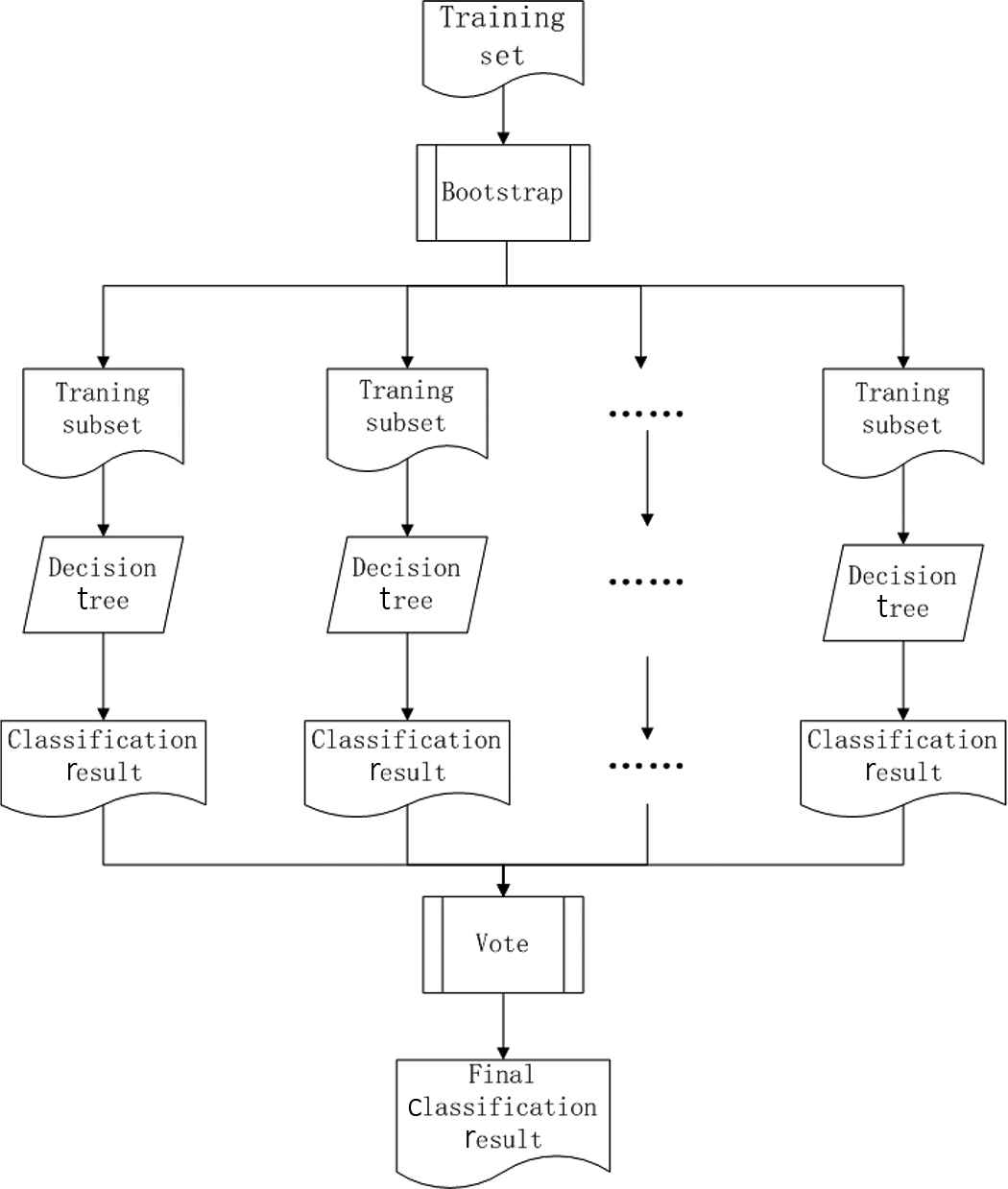
The construction of random forest
The concrete construction process of the decision tree is as follows.
- •
Input the number m of features for each decision tree (m < M);
- •
For each node, select m features randomly, calculate the information gain of each feature, then find the optimal splitting method of the decision tree.
- •
Each decision tree grows according to the training subset without pruning. Finally, we get a decision tree h(x, θ), x denotes the training subset, and θ represents the feature subset.
The random forest has many advantages that make it promising for the problem of classifying the gas users. First of all, random forest has better accuracy compared with other classification algorithms. Furthermore, it has better denoising ability, and it runs efficiently while dealing with large data sets, like gas consumption records, since the process of training is independent among trees.
3. FLOOR HEATING CUSTOMERS PREDICTION USING RANDOM FOREST MODEL
This section uses random forest to build a model for predicting potential customers of floor heating.
3.1. Data Preprocessing
Data preprocessing includes feature extraction and feature processing as follows.
3.1.1. Feature extraction
Due to the significant differences in gas consumption between the users of the floor heating group and those of the non-floor heating group, we extract the gas records of all residents for 3 years from 2014 to 2016. Considering the different meter reading time of gas subsidiary companies, we calculate the usage at the interval of 2 months. The structural feature set is shown in Table 1. The structure of 2015 and 2016 gas consumption features are similar.
| Name | Meaning | Calculation |
|---|---|---|
| Y141 | Gas consumption in 1st period, 2014 | Gas consumption in January and February, 2014 |
| Y143 | Gas consumption in 2nd period, 2014 | Gas consumption in March and April, 2014 |
| Y145 | Gas consumption in 3rd period, 2014 | Gas consumption in May and June, 2014 |
| Y147 | Gas consumption in 4th period, 2014 | Gas consumption in July and August, 2014 |
| Y149 | Gas consumption in 5th period, 2014 | Gas consumption in September and October, 2014 |
| Y1411 | Gas consumption in 6th period, 2014 | Gas consumption in November and December, 2014 |
Feature set of 2014
3.1.2. Feature processing
We constructed 18 features of gas consumption. However, we found that there were both missing and abnormal data in the features after analysis.
The missing data of certain months are caused by the difference in the time when users start to use gas or the deliberate negligence of the gas system. We amend this by supplementing the records of the other 2 years in the same period.
There are several types of abnormal feature data. We deal with them respectively.
3.1.2.1. Negative value
We use default value 0 to replace the negative values in the gas consumption records.
3.1.2.2. Missing values
There are still a large number of missing values in the gas usage records after the replacement. We removed the user from the floor heating group if the number of value 0 is larger than 9 in the 18 features.
3.1.2.3. Misjudgement
The features of some users who belong to the non-floor heating group may conform to the pattern of floor heating users. After analysis and confirmation, the reason is that the operator may have mis-recorded the situation. We handle this in the following way.
- •
If there are more than two feature values larger than the corresponding 75-fractile in the group of floor heating users in 2014, the user category is modified to the category of floor heating users, otherwise go to the next step.
- •
If there are more than two feature values larger than the corresponding 75-fractile in the group of floor heating users in 2015, the user category is modified to the category of floor heating users, otherwise go to the next step.
- •
If there are more than two values larger than the corresponding 75-fractile in the group of floor heating users in 2016, the user category is modified to the category of floor heating users, otherwise go to the next step.
- •
If there are more than three values larger than the corresponding 75-fractile in the group of floor heating users from 2014 to 2016, the user category is modified to the category of floor heating users, then stop.
Taking the six characteristics in 2016 as an example, the quartiles, standard deviations and averages of the training dataset are shown in Table 2, the values of floor heating category dataset are shown in Table 3, and the values of non-floor heating category dataset are shown in Table 4.
| Training set | Min | 25% | 50% | 75% | Max | Average | Standard deviation |
|---|---|---|---|---|---|---|---|
| Y161 | 0 | 11 | 40 | 80 | 18568 | 91.175 | 197.25 |
| Y163 | 0 | 12 | 40 | 81 | 11537 | 89.026 | 187.436 |
| Y165 | 0 | 11 | 33 | 61 | 9041 | 153.75 | 100.96 |
| Y167 | 0 | 10 | 25 | 44 | 6589 | 35.695 | 63.022 |
| Y169 | 0 | 9 | 23 | 40 | 14304 | 31.888 | 66.434 |
| Y1611 | 0 | 11 | 30 | 54 | 7860 | 45.782 | 76.491 |
Min, quartiles, max, average, standard deviation of gas consumption of the residents in training set, 2016
| Floor heating user | Min | 25% | 50% | 75% | Max | Average | Standard deviation |
|---|---|---|---|---|---|---|---|
| Y161 | 0 | 60 | 153 | 408 | 18568 | 294.29 | 371.702 |
| Y163 | 0 | 60 | 154 | 3712 | 5879 | 279.145 | 348.141 |
| Y165 | 0 | 42 | 84 | 159 | 9041 | 134.68 | 196.96 |
| Y167 | 0 | 30 | 53 | 97 | 6589 | 80.89 | 120.79 |
| Y169 | 0 | 25 | 47 | 82 | 14304 | 70.61 | 135.025 |
| Y1611 | 0 | 37 | 71 | 136 | 7860 | 110.723 | 142.707 |
Min, quartiles, max, average, standard deviation of gas consumption of floor heating users, 2016
| Non-floor heating user | Min | 25% | 50% | 75% | Max | Average | Standard deviation |
|---|---|---|---|---|---|---|---|
| Y161 | 0 | 6 | 30 | 60 | 1593 | 42.104 | 50.535 |
| Y163 | 0 | 8 | 32 | 61 | 11537 | 43.095 | 59.134 |
| Y165 | 0 | 8 | 28 | 50 | 2363 | 33.484 | 35.930 |
| Y167 | 0 | 6 | 21 | 36 | 2565 | 24.776 | 28.174 |
| Y169 | 0 | 6 | 20 | 33 | 3481 | 22.532 | 25.007 |
| Y1611 | 0 | 8 | 25 | 44 | 3452 | 30.092 | 32.854 |
Min, quartiles, max, average, standard deviation of gas consumption of non-floor heating users, 2016
3.2. Prediction Model
In the prediction of floor heating customer, features established based on the gas consumption records are used as input, the classification of gas user is the prediction result. The prediction model is obtained through the training set.
Assume that Strain represents the training set with N samples, every sample has M features, the modeling process is as Algorithm 1.
| Input: Training set Strain = (Xi, Yi)|i = 1, 2, …, N}; Factors set |
| I = {(I1, I2, …, IM)}; The number of decision trees k |
| Output: A random forest H |
| 1: function Forest Generate (Strain, I, k) |
| 2: for j = 0 → k – 1 do |
| 3: Strain, j = {(Xi, Yi)|i = 1, 2, …, n} ← Randomly sample the training set with replacement to generate the subset; |
| 4: θj = {θj1, θj2,…, θjm} ← Randomly select m features instead of using M features to split; |
| 5: h(X, θj) ← Generate a decision tree; |
| 6: end for |
| 7: return H = {h(X, θj)| j = 1, 2, ..., k} |
| 8: end function |
The prediction Model
4. EXPERIMENT AND ANALYSIS
4.1. Datasets and Evaluation Metrics
The data sets are based on the real data of gas users are provided in Shanghai. The field I_DINUAN is used to identify customer who are using floor heating. Residents using floor heating is identified by 1, and the others are identified by 0.
After the missing values and abnormal values were processed, the total number of gas users in the dataset is 2,73,415, the number of floor heating users is 53,206, the number of resident users who have been identified as non-floor heating users is 2,20,213. We divided the labeled users into training set and test set in a ratio of 7:3.
The combination of the actual category of the sample and the prediction of classifiers can be divided into four cases: True Positive (TP), False Positive (FP), True Negative (TN) and False Negative (FN). The confusion matrix is shown in Table 5.
- •
False negative (FN) is the sample that is judged as negative but is positive actually.
- •
False positive (FP) is the sample that is judged as positive but is negative actually.
- •
True negative (TN) is the sample that is judged as negative and is negative actually.
- •
True positive (TP) is the sample that is judged as positive and is positive actually.
| Actual condition | |||
|---|---|---|---|
| Actual positive | Actual negative | ||
| Predicted | Predicted positive | True positive (TP) | False positive (FP) |
| Condition | Predicted negative | False negative (FN) | True negative (TN) |
Confusion matrix
As usual for two-class problems in machine learning, the performance of our floor heating customer prediction model is measured using accuracy, precision, recall, F1-score, Receiver Operating Characteristic (ROC) curve and Area Under the Curve (AUC).
Accuracy, as defined in Equation (1), reflects the ability to judge the whole model, that is, the proportion of samples that are correctly predicted. Precision, as defined in Equation (2), reflects the ability to discriminate negative samples. The higher the precision, the stronger ability the method has to differentiate the negative samples. Recall, as defined in Equation (3), reflects the ability to identify positive samples. The higher the recall, the stronger ability the model has to recognize positive samples. F1-score, as shown in Equation (4), is a combination of precision and recall. The higher the F1-score, the more robust the classification model is
In the ROC curve, the abscissa of each point is False Positive Ratio (FPR), and the ordinate is True Positive Ratio (TPR). The definition of FPR is shown in Equation (5), and the definition of TPR is shown in Equation (6). We can get a point (FPR, TPR) based on the performance on the test set. By adjusting the threshold of the classifier, we can get a corresponding ROC curve of this classifier. ROC curve reflects the ability to classify. The closer the ROC curve is to the upper left corner, the better performance of the classifier is. AUC is defined as the area under the ROC curve. The larger the AUC value, the better the prediction effect of the classifier is
4.2. Experiment Result
The experiment consists of two parts: experiment on the effect of different number of decision trees in the random forest, and experiment on the comparison of random forest with logistic regression and KNN.
4.2.1. Effect of number of decision trees in random forest
The number of decision trees in the random forest model is the key to the result of the model. It will directly decide the classification effect and efficiency of the model. With the gradual increase of the number of decision trees, the performance is better, but the training time will increase. So we should find a trade-off between performance and cost.
4.2.1.1. Accuracy
The trend of accuracy is shown in Figure 2. With the increasing number of decision trees, the accuracy of the random forest model shows an increasing trend. Then it will reach a stable state when the number of trees is 19 and the accuracy is 0.943.
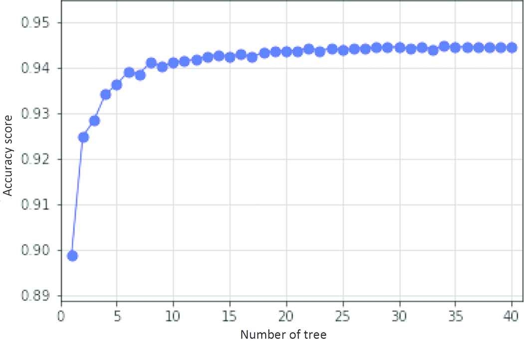
Effect of tree number on accuracy value
4.2.1.2. Precision, recall
The trends of precision and recall are shown in Figure 3. As the number of decision trees in the random forest model increases, the precision and recall value of the model generally increase. When the number of trees is larger than 19, the upward trend is not obvious and tends to be stable. When the number of decision trees reaches 19, it reaches a good state and the precision value is 0.912, the recall value is 0.788.
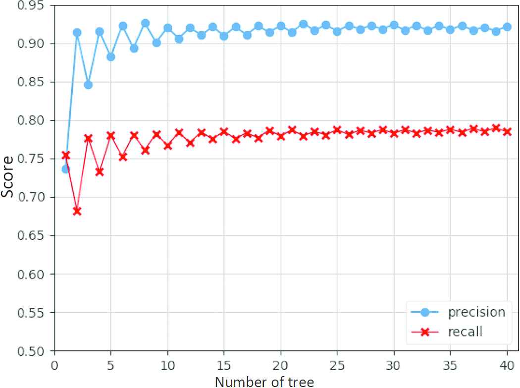
Effect of tree number on precision and recall value
4.2.1.3. F1-score
The change trend of F1-score is shown in Figure 4. The F1-score shows a rising trend when the number of random forest is increasing. The curve tends to be gentle when the number is larger than 19, it will reach a good condition and the F1-score is 0.846 when the number of decision trees is 19.
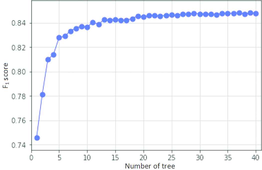
Effect of tree number on F1-score
4.2.1.4. Receiver operating characteristic, area under the curve
The ROC curves and the AUC values are shown in Figure 5. We select the number of decision trees for the random forest model to be 1, 2, 3, 4, and 19 for ROC and AUC calculations. As the number of decision trees increases, the ROC curve of random forest with more decision tree is closer to the upper left corner, and the AUC value of the random forest with more decision trees is also larger. Therefore, it demonstrates that the effect of the prediction will become better as the number of trees is increasing.
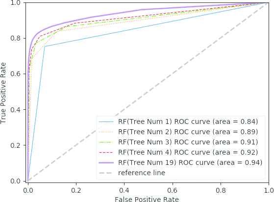
Comparison of ROC curves in random forest model
Based on the above analysis and experiments, we set the number of decision trees in the floor heating prediction model to 19.
4.2.2. Comparative studies
After determining the number of decision trees in the random forest of the floor heating prediction model, we compared the random forest model, logistic regression model and KNN.
4.2.2.1. Accuracy, precision, recall, F1-score
Accuracy, precision, recall and F1-score for the three models are shown in Table 6. From the evaluation results of the four indicators, it can be seen that the performance of the random forest model is relatively the best.
| Classifier | Parameters | F1-score | Precision | Recall | Accuracy |
|---|---|---|---|---|---|
| KNN | k = 5 | 0.7996 | 0.9120 | 0.7118 | 0.9298 |
| LR | Default | 0.6371 | 0.9220 | 0.4867 | 0.8909 |
| RF | n = 19 | 0.8446 | 0.9131 | 0.7857 | 0.9431 |
Comparison of classification results
4.2.2.2. Receiver operating characteristic, area under the curve
The ROC curves and the AUC values of the three models are shown in Figure 6. The ROC curve of the random forest inclined toward the left upper quadrant than those of logistic regression model and KNN model indicating its higher sensitivity and specificity. The AUC value of the random forest, logistic regression, KNN model are 0.94, 0.85, 0.91 respectively. Therefore, it indicates that the random forest has better prediction than logistic regression and KNN.
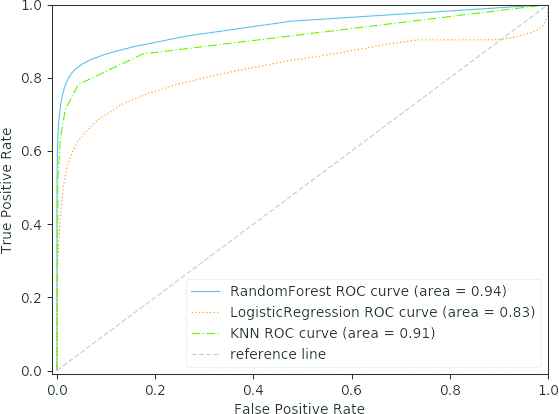
Comparison of ROC curves for random forest, logistic regression and KNN
5. CONCLUSION
This paper presents the application of the random forest for floor heating customer prediction. It can be used to forecast those customers willing to use floor heating. This will help gas companies to provide differentiated services for the customers of the floor heating group, so that the gas companies can maintain their advantages in the fierce competition and increase the economic benefits.
ACKNOWLEDGMENTS
This work is supported by National Natural Science Foundation of China under grants No. 61173048, 61572318, 61702334, 61772200, 61872142, the Information Development Special Funds of Shanghai Economic and Information Commission under Grant No. 201602008, Shanghai Pujiang Talent Program under Grant No. 17PJ1401900, Natural Science Foundation of Shanghai under Grant No. 17ZR1406900, 17ZR1429700, and Educational Research Fund of ECUST under Grant No. ZH1726108.
REFERENCES
Cite this article
TY  - JOUR
AU  - Zhihuan Yao
AU  - Xian Xu
AU  - Huiqun Yu
PY  - 2018
DA  - 2018/12/31
TI  - Floor Heating Customer Prediction Model Based on Random Forest
JO  - International Journal of Networked and Distributed Computing
SP  - 37
EP  - 42
VL  - 7
IS  - 1
SN  - 2211-7946
UR  - https://doi.org/10.2991/ijndc.2018.7.1.5
DO  - 10.2991/ijndc.2018.7.1.5
ID  - Yao2018
ER  -