
Kernel and Range Approach to Analytic Network Learning
- DOI
- 10.2991/ijndc.2018.7.1.3How to use a DOI?
- Keywords
- Least squares error; linear algebra; multilayer neural networks
- Abstract
A novel learning approach for a composite function that can be written in the form of a matrix system of linear equations is introduced in this paper. This learning approach, which is gradient-free, is grounded upon the observation that solving the system of linear equations by manipulating the kernel and the range projection spaces using the Moore–Penrose inversion boils down to an approximation in the least squares error sense. In view of the heavy dependence on computation of the pseudoinverse, a simplification method is proposed. The learning approach is applied to learn a multilayer feedforward neural network with full weight connections. The numerical experiments on learning both synthetic and benchmark data sets not only validate the feasibility but also depict the performance of the proposed formulation.
- Copyright
- © 2018 The Authors. Published by Atlantis Press SARL.
- Open Access
- This is an open access article under the CC BY-NC license (http://creativecommons.org/licences/by-nc/4.0/).
1. INTRODUCTION
The problem of machine learning has been traditionally formulated as an optimization task where an error metric is minimized. In terms of solving the system of linear equations, an approximation is often sought-after according to a least error metric because it is difficult to have an exact match between the sample size and the number of model parameters. Such an approximation to the least error metric, particularly in the squared error form, can be determined analytically either in the primal solution space or in the dual solution space depending on the rank property of the covariance matrix. This optimization approach has been a popular choice due to its simplicity and tractability in analysis and implementation. The approach is predominant in engineering applications as evident from its pervasive adoption in statistical and shallow network learning.
Attributed to the computational effectiveness of the backpropagation algorithm (see e.g. [1–5]) running on the then limited hardware and the theoretical establishment of the mapping capability (see e.g. [6–9]), the multilayer neural networks were once a popular tool for research and applications in the 1980s. With the advancement of computing facilities in the 1990–2000s, such minimization of the error cost function had been progressed to the more memory intensive search algorithms utilizing the first- and the second-order methods of gradient descent (see e.g. [10–12]). Recently, driven by another leap bound advancement in the computing resources together with the availability of a large quantity of data, the multilayer neural networks reemerged as deep learning networks [13]. In view of the demanding task of processing a large quantity of data with the highly complex network function on the limited computing resources such as the operating memory and the level of data vectorization, the backpropagation remained a viable tool for the optimization search.
In this work, we explore into utilization of the kernel and the range space projection for network learning. This approach exploits the approximation property of the column and the row spaces of the system of linear equations for learning the network weights. The main advantage of this approach is that neither descent nor gradient computation is needed for network learning. Moreover, the network learning can be computed analytically where no iterative search is needed. The proposed approach can be applied to networks of arbitrary number of layers. This proposal opens up a new way of solving the network and functional learning problems without having to compute the gradient.
2. PRELIMINARIES
2.1. Kernel and the Range
In engineering applications, it is common to formulate the problem as a system of linear equations given in Equation (1):
For an under-determined system where m < d equations in Equation (1), the number of equations is less than the number of unknown parameters. This gives rise to an infinite number of solutions to the parameters when minimizing the least error cost. However, a least norm solution [14] can be obtained by constraining w ∈ ℝd to the ℝm subspace [15] using ŵ = XTâ where â = (XXT)−1 y. Here, XXT constitutes the kernel and is also known as the Gram matrix.
For an over-determined system where m > d, the m equations in Equation (1) are generally unsolvable when a strict equality is desired (see e.g. [16]). However, by multiplying XT to both sides of Equation (1), the resulted d equations in Equation (2)
Collectively, by denoting X† = (XT X)−1 XT when XT X has full rank and X† = XT (XXT)−1 when XXT has full rank, the above observations can be summarized as follows:
2.2. Moore–Penrose Inverse
The matrix inversion given by X† = (XT X)−1 XT is known as the left inverse and that given by X† = XT (XXT)−1 is known as the right inverse. More generally, for non-square matrices, such matrix inversions can be defined in the form of the Moore–Penrose inverse as follows.
Definition 1
(see e.g. [19,20]) If X (square or rectangular) is a matrix of real or complex elements, then there exits a unique matrix X†, known as the Moore–Penrose inverse or the pseudoinverse of X, such that (i) XX†X = X, (ii) X†XX† = X†, (iii) (XX†)* = XX† and (iv) (X†X)* = X†X.
Properties (i)–(iv) in Definition 1 are known as the Penrose equations. If X has a full rank factorization such that X = FG, then X† = G*(GG*)−1 (F*F)−1 F* satisfies the Penrose equations [19]. In practice, a decomposition of X into FG may not be readily available. For such a case, the left and the right inverses can be adopted with regularization.
The relationship between the system in Equation (1) and the solution form in Lemma 1 implies that multiplying the pseudoinverse of a system matrix to both sides of the system equation boils down to an implicit least squares error approximation. The readers are referred to Toh et al. [21] for greater details regarding the approximation. For linear systems with multiple outputs, the following result (see also e.g. [22]) is observed.
Lemma 2.
(see e.g. [23]) Solving for W in the system of linear equations of the form
Based on the above observations, the inherent least squares error approximation property of algebraic manipulation utilizing the Moore–Penrose inverse shall be exploited in the following section to derive an analytic solution for multilayer network learning that is gradient-free.
2.3. Multilayer Feedforward Network
We consider a multilayer feedforward network of n-layers [24] in this study. Unlike conventional networks, the bias term in each layer is excluded except for the inputs in this representation.
Mathematically, an n-layer network model of h1 - h2- ⋯ -hn−1 - hn structure with linear activation at the output layer can be written in matrix form as shown in Equation (5).
2.4. Invertible Function
In some circumstances, we may need to invert the activation function over the network for solution seeking. For such a case, an inversion is performed through a functional inversion. The inverse function is defined as follows.
Definition 2
Consider a function f which maps x ∈ ℝ to y ∈ ℝ, i.e., y = f(x). Then the inverse function for f is such that f−1(y) = x.
A good example of an invertible function is the trigonometric “tan” function where its inverse is given by “tan−1” (or vice versa). Although many other functions are invertible, the functional pair of f = tan−1 and f −1 = tan shall be adopted as an illustrative example in all our experiments.
3. NETWORK LEARNING
3.1. Theory
We learn a network toward a given target matrix Y ∈ ℝm×q by putting G = Y. Here, each layer of the network can be inverted based upon the functional inverse and the Moore–Penrose inverse as following Equations (6)–(8):
Theorem 1
Given m distinct data samples of d dimension which are packed as X ∈ ℝm×(d+1) with augmentation. Consider the multilayer network (5) with linear activation at the output layer. Then, learning of the network towards the target Y ∈ ℝm×q of q dimension admits the following solutions (12)–(15) to the least squares error approximation:
Proof:
The weight matrices in Equations (9)–(11) appear to be dependent on each other. However, according to the findings in Toh et al. [21,23], they can be decoupled based on a random initialization. Here, since the weight matrices W2 ⋯ Wn in Equation (9) consist of random entries during initialization, we can simply put W1 = X† with an implicit identity matrix initialization as a particular choice of the random matrix [24]. Then, weight matrix of the second layer can be found as W2 = [f(XW1)]† which can be written as W2 = [f(XX†)]† since W1 = X†. The setting of the subsequent weights can be obtained from a recursive replacement of X by f(XX†) in each of the layer learning from layer 2 to layer n − 1.
The subsequent step is to replace the pseudoinverse operations in layers 1, ⋯, (n − 1) by a scaled transposition. Suppose the replacement is achieved by putting X† = XT R1 for layer 1, then pre-multiplying both sides by {X}, implies that R1 = (XXT)−1XX† = (XXT)−1 when XXT is invertible. On the other hand, when XT X is invertible, the scaling matrix can be obtained from putting X† = S1 XT which implies that S1 = X† X(XT X)−1 = (XT X)−1. In other words, Rk and Sk, k = 1, ⋯, n − 1 correspond to the inverse terms in the right inverse and in the left inverse of X respectively. Hence the proof.
3.2. Algorithm
For simplicity, consider only the solution based on the right inverse using Rk, k = 1, ⋯, n − 1 in Equation (12) for the algorithmic design. The proposed algorithm for analytic network learning (called ANnet) is summarized as follows:
| Algo. | : ANnet |
|---|---|
| Initial. | : (a) Assign random weights to Rk ∈ ℝm×hk, k = 1, ···, n – 1 in (12)–(14) with arbitrary hk, k = 1, ···, n – 1. |
| (b) Remove Rk, k = 1, ···, n – 1 in (12)–(14) and normalize XT and subsequent composition terms using norm (X). | |
| Learning | : Compute the network weights W1, ..., Wn sequentially using (12)–(15) with the common activation function f = tan–1. |
| Output | : Compute the network output G according to (5). |
The algorithm has two settings. ANnet(a) constitutes the generic algorithmic setting where the number of hidden nodes (given by hk, k = 1, …, n − 1, which are the column sizes of Wk, k = 1, …, n − 1) can be chosen arbitrarily. ANnet(b) is equivalent to assigning identity matrices (of size m × m) to Rk, k = 1, …, n − 1 so that no initialization is needed. This assignment could incur large size of operating memory when the data sample size (m) is large. To facilitate appropriate numerical scaling in such a case, the data matrices XT, f(XXT)T, … in each layer are divided by norm (X).
4. SYNTHETIC DATA
In this section, we observe the behavior of the proposed network learning on three synthetic data sets with known properties. The first set of data represents the regression problem whereas the second and third data sets are well-known benchmarks for classification.
4.1. Single Dimensional Regression Problem
The first set of synthetic data has been generated using y = sin(2x)/(2x) based on x ∈ {1, 2, 3, 4, 5, 6, 7, 8} for training. To simulate noisy outputs, a 20% of variation from the original y values has been incorporated. A total of 10 trials of such noisy measurements are included for training apart from the original signal. A two-layer ANnet(b) is adopted to learn the augmented data (i.e., input with bias). Figure 1a shows the learning results for all the 11 sets of training data. Since there are eight data samples for each training set, the structure of ANnet(b) is 8-1 where the number of hidden nodes is equal to the number of samples. The results for these 11 target functions (one original, plus 10 noisy ones) show fitting of all data points for all the curves. Figure 1b shows the results when a five-layer ANnet(b) (i.e., a 8-8-8-8-1 structure) is adopted. This result shows under-fitting of the data points.
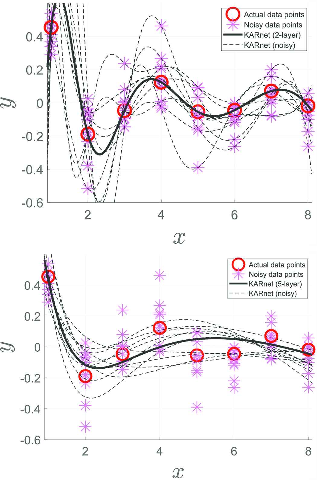
(a) Decision outputs of a two-layer ANnet(b). (b) Decision outputs of a five-layer ANnet(b)
Comparing the two cases, the network is seen to find its fit through all data points including those noisy ones for the two-layer network. However, the five-layer network does not fit every data points. This is due to the inherent deficiency in range projection in ANnet(b) where the pseudoinverse operation has been replaced by a scaling. This example illustrates the fitting behavior of the proposed multilayer network learning based on ANnet(b).
4.2. XOR Problem
The next example is the well-known XOR problem which consists of four data points (i.e., the input data points are {(0, 0), (1, 1), (1, 0), (0, 1)} which are associated with labels {0, 0, 1, 1} respectively). A two-layer ANnet(b) with four hidden nodes is adopted to learn the augmented data (i.e., input with bias giving {(1, 0, 0), (1, 1, 1), (1, 1, 0), (1, 0, 1)}). For comparison, the feedforwardnet of the Matlab toolbox is adopted with a similar architecture (adopting a two-layer structure with tan−1 activation) for learning the same set of data using the default training method trainlm. Figure 2a and b shows respectively the learned decision surfaces for ANnet(b) and feedforwardnet. These results show the capability of ANnet(b) to fit the nonlinear surface and the premature stopping of feedforwardnet at local minimum for this data set.
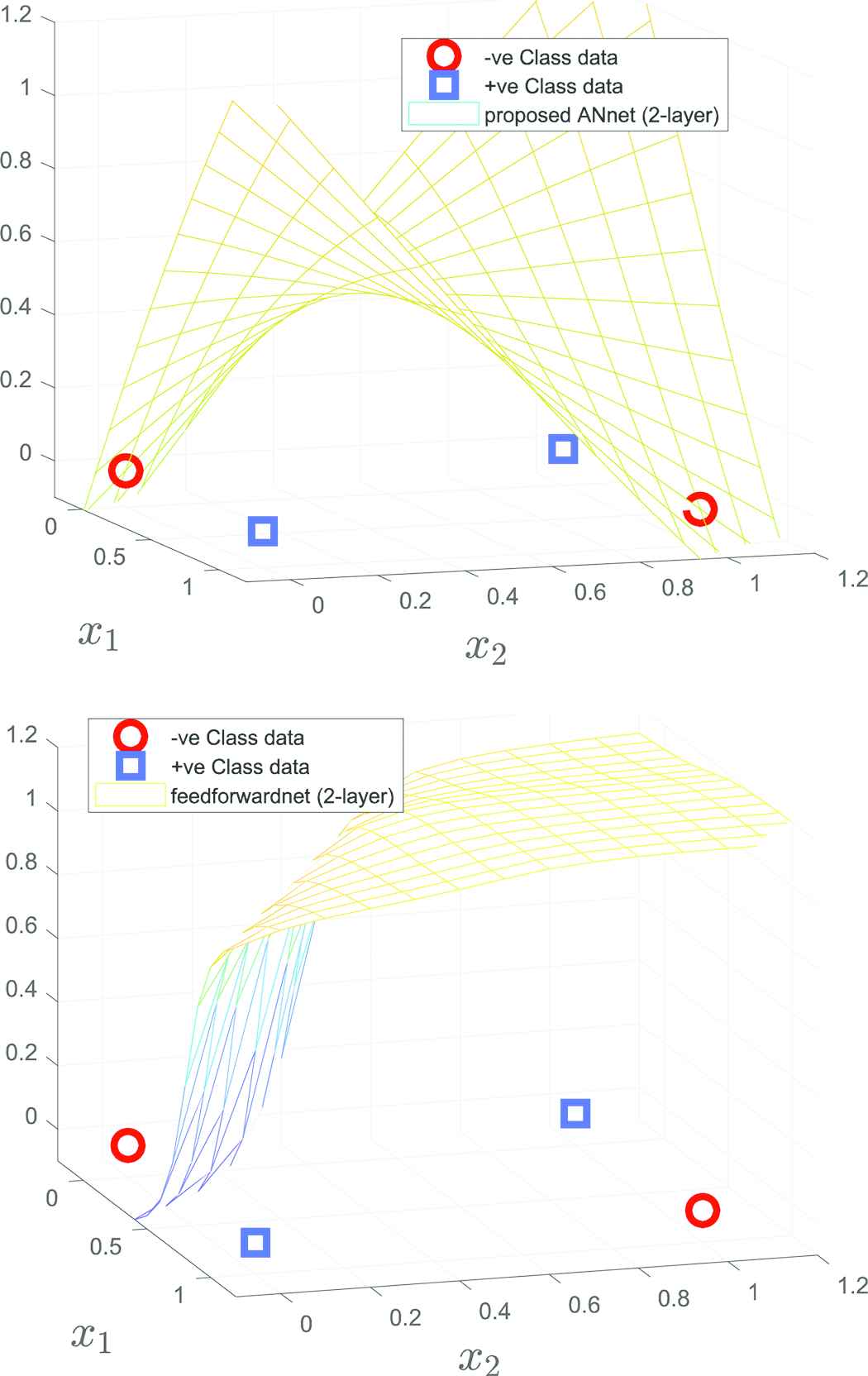
Decision surfaces of two-layer feedforward networks (ANnet(b) and feedforwardnet both using f = tan−1 activation, feedforwardnet was trained by trainlm)
Next, we compare the two networks using a five-layer architecture with each layer having four hidden nodes for both networks. Figure 3a and b shows respectively the decision surfaces for ANnet(b) and feedforwardnet. These results show the fitting capability of ANnet(b) despite the larger number of adjustable parameters and again, the premature stopping of feedforwardnet for this data set.
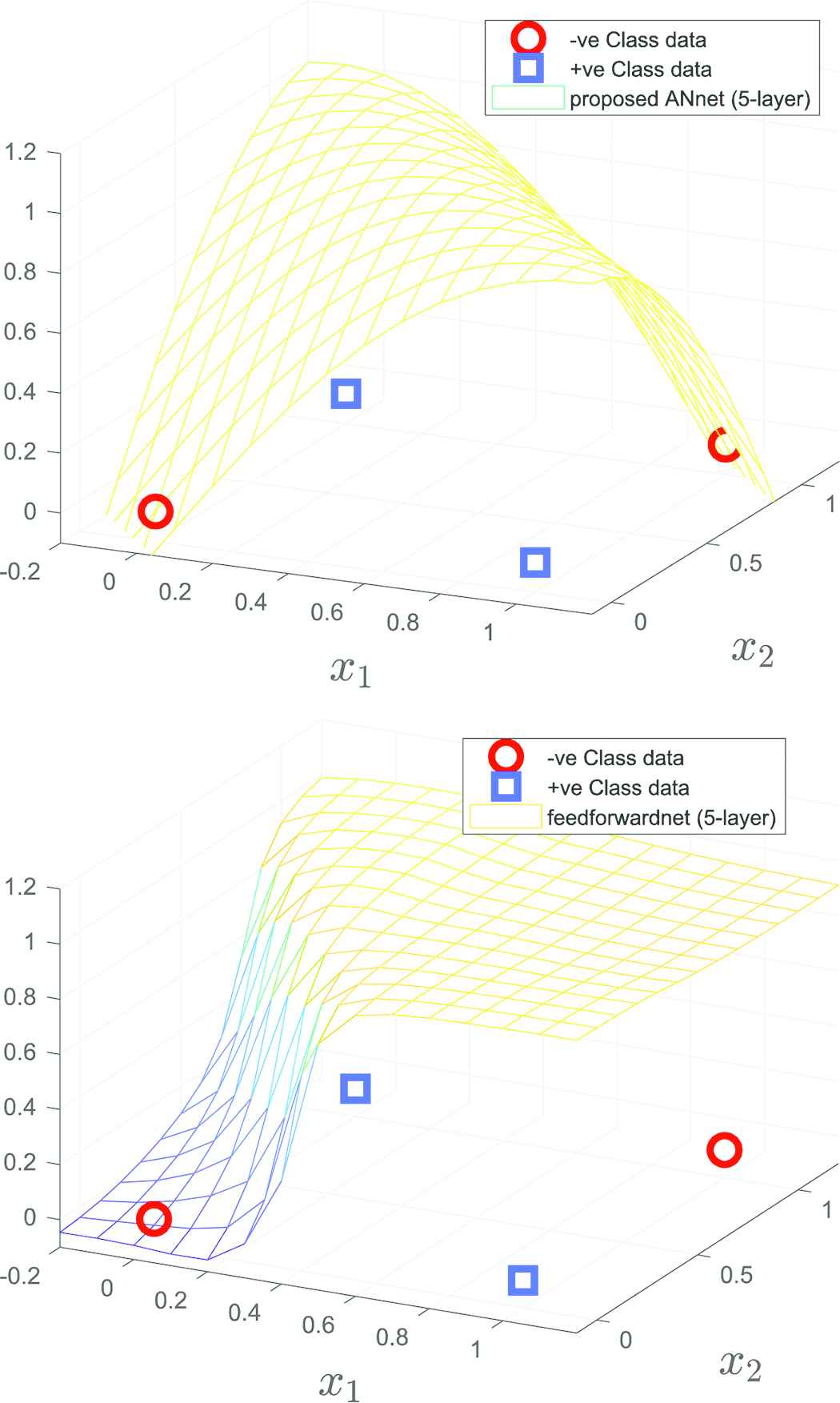
Decision surfaces of five-layer feedforward networks (ANnet(b) and feedforwardnet both using f = tan−1 activation, feedforwardnet was trained by trainlm)
4.3. Three-Spiral Problem
In this example, a total of 1500 randomly perturbed data points which form a three-spiral distribution have been used as the training data. Among these data, each of the spiral arm consists of 500 data points (which are shown as red, green and blue circles in Figure 4). A three-layer ANnet(b) with 1500 hidden nodes at each layer has been adopted for learning these data points with respective labels using an indicator matrix. Since there are three classes, the number of output nodes is 3. The learned decision regions (which are shown in light red, green and blue tones) as shown in Figure 4 shows the mapping capability of ANnet(b) for the three-category problem.
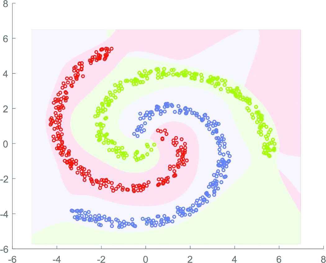
Decision regions of ANnet(b) of three layers
5. EXPERIMENTS ON REAL-WORLD DATA
The experiments are conducted in two parts. In the first part, four data sets of medium sample size (ranging from 5620 to 20,000 sample sizes) from the UCI Macine learning repository [25] are adopted for this experimentation. The proposed learning algorithms ANnet(a) and (b) are experimented in this study based on 10 trials of 10-fold cross-validation tests. The results are reported in terms of the average accuracies of the test sets. The accuracy is defined as the percentage of samples being classified correctly. In the second part, two benchmark data sets from the deep learning literature are experimented. The evaluating protocol follows the hold-out test according to the benchmark.
5.1. UCI Data Sets
For the two-layer ANnet(a), the size of the hidden nodes (i.e., h1, which corresponds to the column size of the hidden layer matrix) is chosen based on an inner 10-fold cross-validation loop using only the training set among h1 = h ∈ {1, 2, 3, 5, 10, 20, 30, 50, 80, 100, 200, 500}. For the three-layer ANnet(a), a network structure of 2h-h-q is adopted where q is the output dimension. The chosen hidden node size is then applied for 10 runs of test evaluations using the outer cross-validation loop.
For ANnet(b), the network structure is inherently fixed according to the data sample size (i.e., h1 = m for the two-layer network and h1 = h2= m for the three-layer network. The size of hidden nodes at the output layer is q for both networks.)
The computing platform for the experiments in part-one is a notebook computer with an Intel i7-6500U CPU running at 2.59 GHz. The system has 8 GB of RAM memory.
5.1.1. Nursery data set
The goal in this database [25,26] was to rank applications for nursery schools based upon attributes such as occupation of parents and child’s nursery, family structure and financial standing, as well as the social and health picture of the family. The eight input features for the 12,960 instances are namely, ‘parents’ with attributes usual, pretentious, great_pret; ‘has_nurs’ with attributes proper, less_proper, improper, critical, very_crit; ‘form’ with attributes complete, completed, incomplete, foster; ‘children’ with attributes 1, 2, 3, more; ‘housing’ with attributes convenient, less_conv, critical; ‘finance’ with attributes convenient, inconv; ‘social’ with attributes non-prob, slightly_prob, problematic; ‘health’ with attributes recommended, priority, and not_recom. These input attributes are converted into discrete numbers and normalized to the range (0, 1]. The output decisions include ‘not_recom’ with 4320 instances, ‘recommend’ with two instances, ‘very_recom’ with 328 instances, ‘priority’ with 4266 instances and ‘spec_prior’ with 4044 instances. Since the category ‘recommend’ has not enough instances for partitioning in 10-fold cross-validation, it is merged into the ‘very_recom’ category. We thus have four decision categories for classification.
The average accuracies for the two-and three-layer ANnet(a) are respectively 92.01% at h = 500 and 89.03% at h = 80. These results are lower than 98.89% for the feedforwardnet (h = 100, two-layer) and comparable with 91.69% for the total error rate method adopting RM model (TERRM) method [27]. For ANnet(b), the average accuracies are respectively 95.67% and 92.19% for the networks of two- and three-layers.
5.1.2. Letter recognition
The data set comes with 20,000 samples, each with 16 feature attributes. The goal is to recognize the 26 capital letters in the English alphabet based on a large number of black-and-white rectangular pixel displays. The character images consist of 20 different fonts where each letter within these 20 fonts was randomly distorted to produce a large pool of unique stimuli [25,28]. Each stimulus was converted into 16 primitive numerical attributes such as the statistical moments and the edge counts. These attributes were then scaled to fit into a range of integer values from 0 to 15.
The average accuracies for the two-and three-layer ANnet(a) are respectively 90.38% and 52.33%, both at h = 500. The results for ANnet(b) are 91.79% and 69.29% respectively for the two-and three-layer networks. The feedforwardnet (two-layer) encountered “out of memory” for the computing platform of Intel i7-6500U CPU at 2.59 GHz with 8 GB RAM.
5.1.3. Optical recognition of handwritten digits
This data set was collected based on a total of 43 people, wherein 30 of them contributed to the training set and the remaining 13 to the test set [25,29]. The original 32 × 32 bitmaps were divided into non-overlapping blocks of 4 × 4 where the number of on pixels were counted within each block. This generated an input matrix of 8 × 8 where each element was an integer within the range [0, 16]. The dimensionality (64) is thus reduced (from 32 × 32) and the resulted image is invariant to minor distortions. The total number of samples collected for training and testing are respectively 3823 and 1797. In our experiment, these two sets (training and test sets) of data are combined for the running of 10 trials of 10-fold cross-validation tests. Figure 5 shows some samples of the reduced resolution image taken from the training set (upper two panels) and the testing set (bottom two panels).
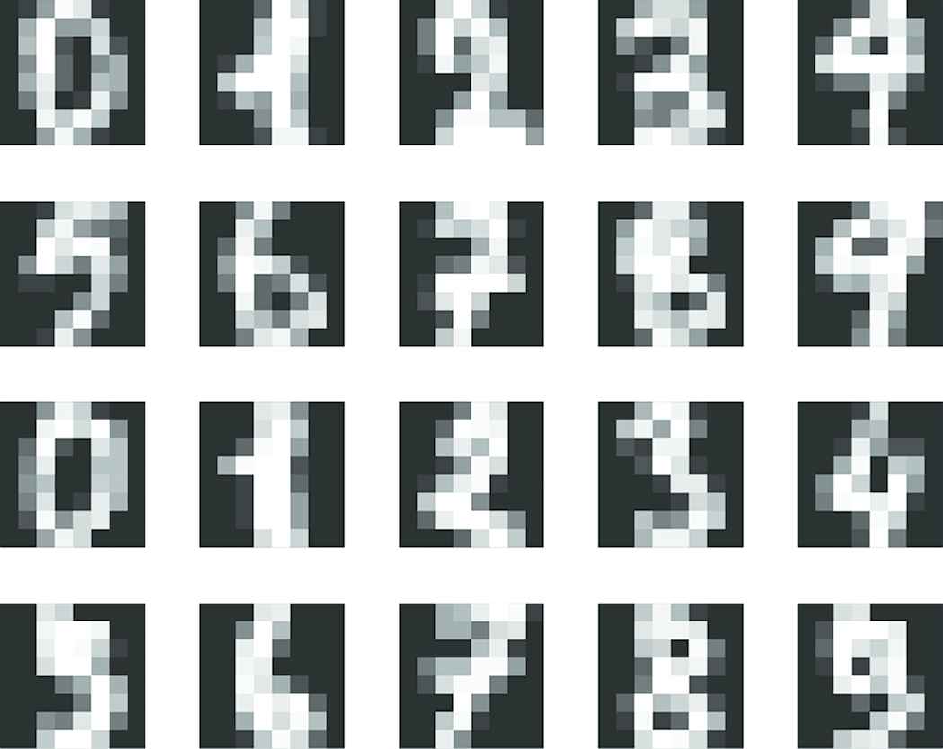
Handwritten digits: samples in the upper two panels are taken from the training set and samples in the bottom two panels are taken from the test set
The average accuracies for the two-and the three-layer ANnet(a) are respectively 97.41% at h = 500 and 93.69% at h = 500. These results are comparable with the 96.81% for the TERRM method [27] and the 98.16% for the TERRP method [30]. The ANnet(b) shows 96.82% and 99.06% accuracies respectively for the two-and three-layer structures. These results are comparable with that of support vector machines radial basis function (SVM-Rbf) with 99.13% recognition accuracy. The feedforwardnet (two-layer) encounters “out of memory” for the current computing platform.
5.1.4. Pen-based recognition of handwritten digits
This data set was collected based on the handwritten digits on a pressure sensitive tablet with an integrated LCD display and a cordless stylus from 44 writers [25,31]. The writers were asked to write 250 digits (0–9) in random order inside boxes of 500 × 500 tablet pixel resolution. A total of 10,992 digit samples formed the entire database for recognition. The original 500 × 500 table pixel resolution was re-sampled to form a feature length of 16. No sample data is display here due to the very low image resolution of 4 × 4. Similar to other data sets, we perform 10 trials of 10-fold cross-validation tests for this data set.
The average accuracies for the two-and three-layer ANnet(a) are respectively 98.88% (h = 500) and 91.94% (h = 500). For ANnet(b), the accuracies for the two-and three-layer networks are respectively 99.54% and 98.36%. These results show competing accuracy with TERRM, TER-RP and SVM-Rbf.
5.1.5. State-of-the-arts comparison
The state-of-the-art methods adopted for comparison are namely, the reduced multivariate (RM, [32]) polynomial method, the TERRM [27], the feedforwardnet (two-layer) from the Matlab toolbox [33], the SVM adopting polynomial (SVM-Poly, [34]) kernel and SVM radial basis function (SVM-Rbf, [34]) kernel, all running under the same protocol of 10 trials of 10-fold cross-validation tests.
Table 1 shows that the proposed ANnet has comparable prediction accuracy with the compared state-of-the-art methods. While the SVMs have been tuned by adjusting the kernel parameters (such as the order in the polynomial kernel and the Gaussian width in the radial basis kernel), the proposed network ANnet(a) has been tuned by adjusting the number of hidden nodes (h) in each layer according to the structures h-q and 2h-h-q. The network ANnet(b) has a default setting of the hidden node size according to the data sample size. The results show competence of the proposed ANnet(a),(b) with state-of-art classifiers for medium sample size data sets of relatively small dimension.
| Methods | Nursery | Letter | Optdigit | Pendigit |
|---|---|---|---|---|
| RM [32] | 90.93 | 74.14 | 95.32 | 95.73 |
| TERRP [30] | 96.46 | 88.20 | 98.16 | 99.27 |
| TERRM [27] | 91.69 | 78.42 | 96.81 | 97.28 |
| SVM-Poly [34] | 91.61 | 77.22 | 95.52 | 94.50 |
| SVM-Rbf [34] | 98.24 | 97.14 | 99.13 | 99.52 |
| FFnet(2L) [33] | 98.89 | OM | OM | OM |
| ANnet(a)-2L | 92.01 | 90.38 | 97.41 | 98.88 |
| ANnet(a)-3L | 89.03 | 52.33 | 93.69 | 91.94 |
| ANnet(b)-2L | 95.67 | 91.79 | 96.82 | 99.54 |
| ANnet(b)-3L | 92.19 | 69.29 | 99.06 | 98.36 |
OM: out of memory for the current computing platform, 2L, 3L: two-and three-layer respectively, FFnet: Feedforwardnet from Matlab [33].
Comparison of accuracy (%) with state-of-the-arts
5.2. MNIST and CIFAR10 Data Sets
In deep learning, the MNIST [35,36] and the CIFAR10 [37,38] data sets are among those popular benchmark image data sets for algorithmic study and experimental comparison. The MNIST database of handwritten digits contains a training set of 60,000 samples and a test set of 10,000 samples where each sample image is of 28 × 28 pixels size. The CIFAR10 database of objects consists of a training set of 50,000 samples and a test set of 10,000 samples where each image in each of the three RGB channels is of 32 × 32 pixels size. Each image sample thus contains 3 × (32 × 32) = 3072 pixels in total. In this study, every image is sub-sampled into 3 × (8 × 8) = 192 pixels for the three channels. Both of these data sets have an output of 10 class labels (i.e., q = 10). Different from the above cross-validation protocols, we follow the commonly adopted protocol of hold-out test in the deep learning community in this study. Figures 6 and 7 show respectively some training and test sample images from the MNIST and CIFAR10 data sets.
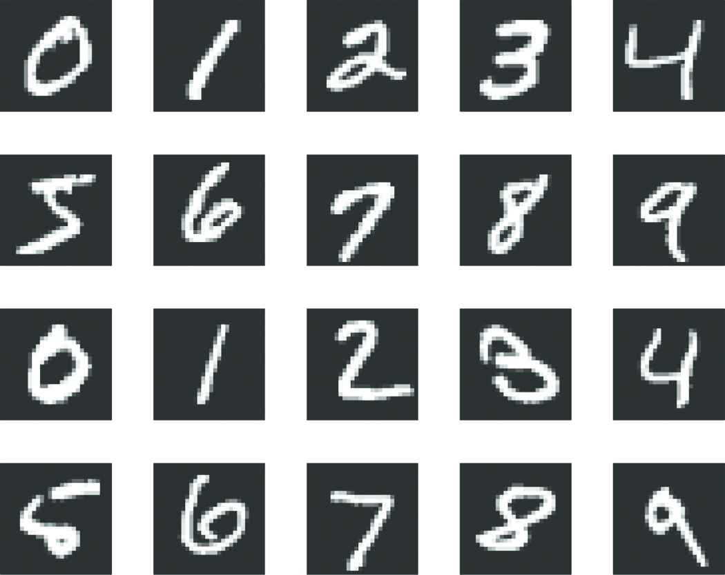
MNIST data set: samples in the upper two panels are taken from the training set and samples in the bottom two panels are taken from the test set
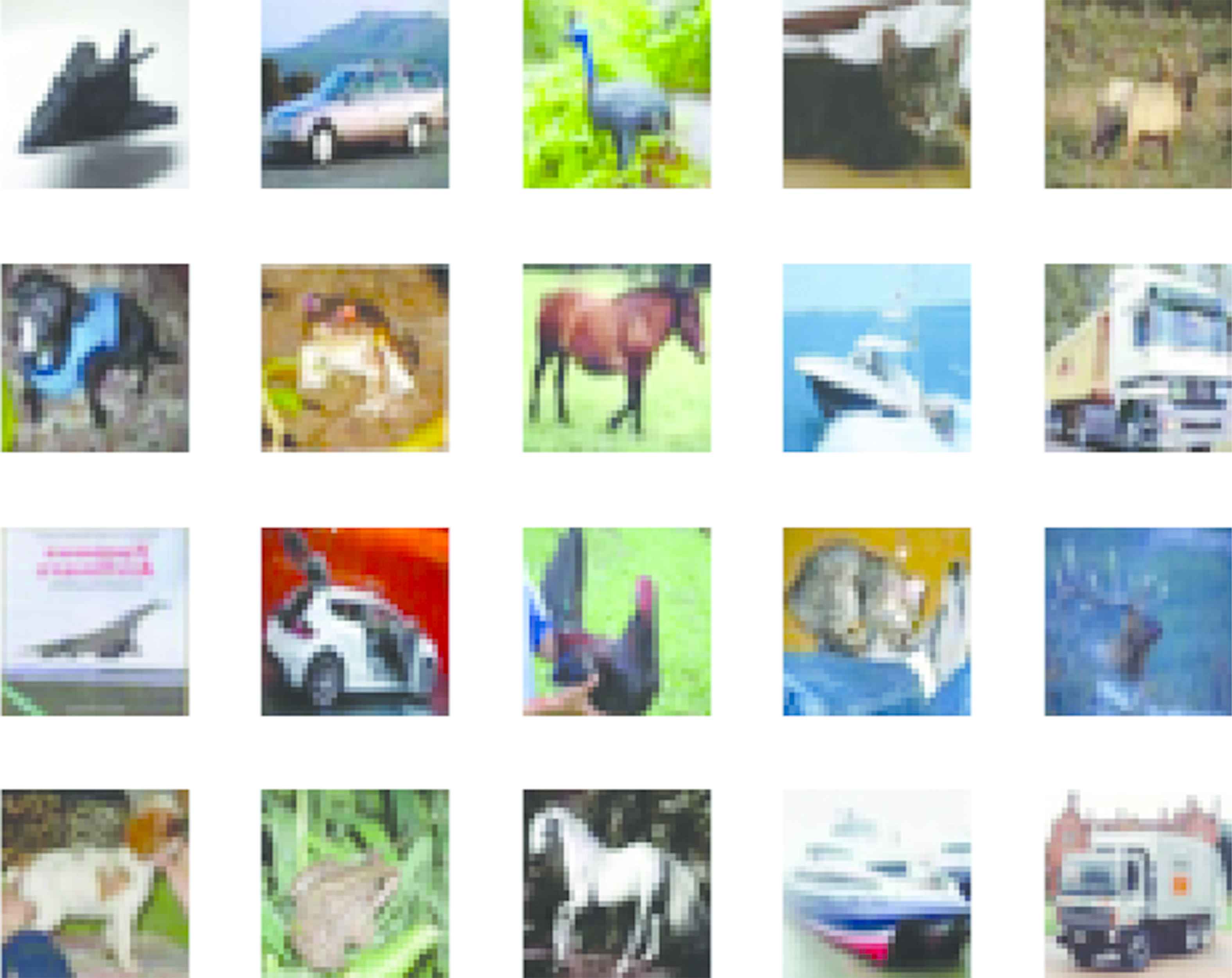
CIFAR10 data set: samples in the upper two panels are taken from the training set and samples in the bottom two panels are taken from the test set
The computing platform for the experiments in part-two is a computer with an Intel i7-7820X CPU running at 3.60 GHz. The system has 96 GB of RAM memory. The training CPU time is measured using the Matlab’s function CPU time which corresponds to the total computational times from each of the 8 cores in the Processor. In other words, the physical time experienced is about 1/8 of this clocked CPU time.
The training and test results of ANnet(a) and (b) of two-layers for MNIST data set are shown in Table 2 with respective training CPU processing times. For ANnet(a), the test accuracy is seen to be increasing with the number of the hidden layer nodes. However, such increment trend of the accuracy is observed to peak at 5000 hidden nodes and starts to decline beyond. This is apparently an over-trained case for a fully connected network with large number of hidden nodes.
| ANnet structure | Training | Test | CPU (s) |
|---|---|---|---|
| Linear-classifier | 85.77 | 86.03 | 18.1719 |
| (a): 1000-10 | 91.70 | 91.41 | 43.6094 |
| (a): 5000-10 | 94.49 | 92.70 | 717.0938 |
| (a): 10000-10 | 95.54 | 92.56 | 3271.2343 |
| (a): 27000-10 | 97.64 | 90.74 | 34111.0313 |
| (b): 1000-10 | 94.30 | 94.37 | 29.1719 |
| (b): 5000-10 | 98.17 | 97.25 | 701.2500 |
| (b): 10000-10 | 99.22 | 97.85 | 3227.0625 |
| (b): 27000-10 | 99.93 | 98.24 | 37267.9844 |
MNIST: classification accuracy (%) and training CPU time (s)
For ANnet(b), the hidden layer weight matrix W1 has been set according to a condensed feature matrix instead of the full data matrix due to insufficient computational memory. The condensed feature matrix was obtained by summing the feature vectors over a regular interval such that the resultant sample size (the row size of X) is reduced for W1’s column size setting. Under this setting, the results show comparable test accuracy with state-of-the-arts at high condensed feature size.
With similar settings as that in the above experiments, the training and test results of ANnet(a) and (b) for CIFAR10 data set are tabulated in Table 3 with respective training CPU processing times. Due to the large variation of images between those in the training set and those in the test set, the accuracy only shows a 10% improvement from that of the linear classifier for ANnet(b). These results show insufficiency of the fully connected network for this application.
| ANnet structure | Training | Test | CPU (s) |
|---|---|---|---|
| Linear-classifier | 40.59 | 40.15 | 1.6719 |
| (a): 1000-10 | 39.58 | 38.66 | 24.1718 |
| (a): 5000-10 | 42.37 | 39.13 | 573.8594 |
| (a): 10000-10 | 43.94 | 39.44 | 2800.4375 |
| (a): 25000-10 | 47.63 | 39.16 | 24423.1718 |
| (b): 1000-10 | 50.42 | 47.13 | 23.2656 |
| (b): 5000-10 | 65.15 | 50.58 | 608.5000 |
| (b): 10000-10 | 75.99 | 49.90 | 2746.2031 |
| (b): 25000-10 | 88.37 | 46.93 | 37514.9688 |
CIFAR10: classification accuracy (%) and training CPU time (s)
6. CONCLUSION
By exploiting the observation that a manipulation of the kernel and the range space boils down to the least squares error approximation, a gradient-free learning approach was proposed for multilayer network learning. In order to reduce the computational complexity of the pseudoinverse of data matrix within the hidden-layers, a simplified matrix scaling was introduced. The learning results of synthetic and real-world data provided not only the numerical evidence but also insights regarding the learning mechanism. This opens up the vast possibilities along the research direction.
ACKNOWLEDGMENTS
This research was supported by Basic Science Research Program through the National Research Foundation of Korea (NRF) funded by the Ministry of Education, Science and Technology (Grant number: NRF-2018R1D1A1A09081956).
REFERENCES
Cite this article
TY  - JOUR
AU  - Kar-Ann Toh
PY  - 2018
DA  - 2018/12/31
TI  - Kernel and Range Approach to Analytic Network Learning
JO  - International Journal of Networked and Distributed Computing
SP  - 20
EP  - 28
VL  - 7
IS  - 1
SN  - 2211-7946
UR  - https://doi.org/10.2991/ijndc.2018.7.1.3
DO  - 10.2991/ijndc.2018.7.1.3
ID  - Toh2018
ER  -