
Discrete Differential Evolution Algorithm with the Fuzzy Machine Selection for Solving the Flexible Job Shop Scheduling Problem
- DOI
- 10.2991/ijndc.2018.7.1.2How to use a DOI?
- Keywords
- Fuzzy set; fuzzy selection; flexible job shop; differential evolution; scheduling
- Abstract
The objective of the research is to solve the flexible job shop scheduling problem (FJSP). In this paper, the new algorithm is proposed mainly based on discrete concepts of the differential evolution (DE) algorithm with the new idea called the fuzzy machine selection approach. In the first step, the initial population is created by using a set of the population generation rules. The second step, the arithmetic swapping operation is applied to search for the new operation sequence. In addition, the fuzzy machine selection is utilized to select the proper machine according to the number of operation load and the machine processing time load. Next, the precedence preserving order-based crossover (POX) and the uniform crossover operation are used to enhance the exploitation capability in the third step. The fuzzy machine selection approach embedded the new criteria is used in the local search process to explore the neighbor solution in the surrounding areas of the best 10% of all solutions. The comparative result shows the best performance of the proposed algorithm when compared with the other comparison algorithms.
- Copyright
- © 2018 The Authors. Published by Atlantis Press SARL.
- Open Access
- This is an open access article under the CC BY-NC license (http://creativecommons.org/licences/by-nc/4.0/).
1. INTRODUCTION
At the present, the government encourages entrepreneurs used the innovation and digital technology for enhanced the competitiveness and increased the productivity. To success with the mention above, the entrepreneurs need to adopt the intelligence of the computer in the business. As well as the manufacturing industry, the one important in the manufacturing is to schedule the job plan or the scheduling plan. Nowadays, the industry applied the computer to calculate the schedule and hold the machine balancing in the manufacturing process. The Flexible Job Shop Scheduling Problem (FJSP) is the complex problem which is found in the manufacturing processes. This problem occurs when the staff cannot maintain a balance between the jobs and the machines. In recent years, the researcher in the operation research areas attends to create the metaheuristic algorithm for solving the FJSP. The differential evolution (DE) algorithm is one of the computational algorithms which used to solve the operation research optimization problem. There are several research works which have been proposed; for instance. Mohamed et al. [1] applied the DE algorithm for solving unconstrained global optimization problems. In this algorithm, their proposed a new directed mutation rule based on the weighted difference vector between the best and the worse solution. The local search is utilized to enhance the search capability and to increase the convergence rate. Furthermore, a dynamic non-linear increased crossover probability scheme is proposed balance between the diversity and the convergence rate or between global exploration ability and local exploitation. The result of their algorithm indicates that the improved algorithm outperforms and is superior to other existing algorithms. Salehpour et al. [2] developed the new version of the DE algorithm with the fuzzy logic inference system. This paper uses a fuzzy logic inference system to dynamically tune the mutation factor of DE and improve its exploration and exploitation. A fuzzy system used to considering the variation, namely, number of generation and population. The results obtained show the really good behavior of the proposed method and comparison. Zou et al. [3] presented a Novel Modified Differential Evolution (NMDE) algorithm to solve constrained optimization problems. This algorithm modifies the scale factor of the original DE algorithm by an adaptive strategy. In the crossover operation of this paper, they use the uniform distribution when the stagnation happens to the solution. Moreover, a common penalty function method adopted to balance objective and constraint violations. Experimental results show that the NMDE algorithm has higher efficiency than the other methods in term of finding better feasible solutions of most constrained problems. Huang and Huang [4] proposed the DE algorithm with the ant system for solving the Optimal Reactive Power Dispatch (ORPD) problem. The purpose of ORPD is to reduce active power transmission losses and improve the voltage profile in the power systems. The step of this paper follows the original of DE algorithm. In the mutation process, this paper avoids falling into local minima and save more computational time by using the variable scaling mutation. They test the performance of the proposed algorithm on the IEEE 30-bus system. The experiment shown that, this paper obtains better results with lower active power transmission losses and faster convergence performance than the basic DE methods. Wu and Che [5] proposed a Memetic Differential Evolution (MDE) algorithm for solving the unrelated parallel speed scaling machine scheduling problem. The MDE algorithm improves the basic DE algorithm by using the adaptive meta-Lamarckian learning strategy to integrate the speed adjusting heuristic and job-machine swap heuristics as the local search. The incorporate of these two approaches is to balance the global exploration and local exploitation. The computational results have shown that, their proposed algorithm can significantly improve the basic DE algorithm. Zhang et al. [6] solved a distributed blocking flow shop scheduling problem by introducing the novel hybrid Discrete Differential Evolution (DDE) algorithm. In this paper, they use the heuristic for providing better initial solutions. The mutation and crossover are redesigned to adjust the DDE to the discrete permutations. Last, an effective speedup technique is designed to enhance the algorithmic efficiency. The comparison with the existing algorithms shows their performance.
In our research, a DDE algorithm with the new idea called the fuzzy machine selection is proposed. First, the initial population is generated by the population generation rules. Second, the arithmetic swapping operation and the fuzzy machine selection with the machine load criteria is utilized in the mutation process. Third, we applied the crossover operation to search for the promise solution in the neighboring areas of the target solution. At last, the fuzzy machine selection with the free time criteria is used. The performance of the proposed algorithm is tested with the standard data set.
The remainder of this paper is organized as follows. In Section 2, the FJSP is briefly presented. The original of the DE algorithm is explained in Section 3. In Section 4, the proposed algorithm is demonstrated. Section 5 shows the results, and the final part is the conclusion.
2. FLEXIBLE JOB SHOP SCHEDULING PROBLEM
The FJSP is categorized into the non-deterministic polynomial time hardness problem (NP-hard problem). This problem is found in the manufacturing planning process, for example, the auto parts assembly industries which consist of the precedence jobs and lots of machines that work similarly.
Hence, the objective of the FJSP is to schedule a set of N jobs J = {J1, J2, J3 … JN} on a set of K similarly machines M = {M1, M2, M3 … MK}. The details of the FJSP are, each job may have a different number of operations and each operation can operate with only one machine from the candidate set.
In addition, the processing time of each operation may be different when processed by the different machine. To accomplish solving the FJSP, the following rules are taken into account: (a) each job is independent with others; (b) the operation sequence of each job is arranged according to their precedence; (c) each operation of each job can be processed with only one machine.
Table 1 shows the example of the FJSP. The job J1 contains the three operations as follows, O11 instance represents the first operation of job number one which allowed to be processed by the machine number 1 (M1) and the machine number 3 (M3). The completion time of O11 with the machine M1 is 5 units of the processing time and the completion time of O11 with the machine M3 is 4 units of the processing time. The second operation is O12, to be processed by the machine M1, M2 and M3. The completion tine of the operation O12 on each machine is 4, 2 and 3 units of the processing time respectively. The third operation of job J1 represented by O13 instance, can be processed by all machines; each machine requires a different amount of processing time as follows: the completion time of O13 with the machine M1 is 4 units of processing time. The completion time of O13 with the machine M2 is 2 units of processing time. When applied the O13 to the machine M3 used the 3 units of processing time. Similarly details with the other jobs.
| Job | Operation | Machines | ||
|---|---|---|---|---|
| M1 | M2 | M3 | ||
| J1 | O11 | 5 | – | 4 |
| O12 | 2 | 2 | 5 | |
| O13 | 4 | 2 | 3 | |
| J2 | O21 | 3 | – | – |
| O22 | – | 2 | 1 | |
| J3 | O31 | 3 | 1 | – |
| O32 | 3 | – | 2 | |
The example of the FJSP
3. THEORY BACKGROUND OF THE PROPOSED ALGORITHM
Some aspects of theory background are described below in detail.
3.1. Differential Evolution Algorithm
The DE algorithm is an effective-based evolution algorithm developed by Storn and Price [7] for solving discrete and continuous optimization problem. DE is one of the best genetic type algorithms. The DE is solving a problem by creating new candidate solutions. According to its functionality, the new one is produced by changing the existing ones. At the same time, keep whichever the candidate solution which the best fitness on hand. This algorithm consists of four stages of the procedure: initial population, mutation, reproduction and selection.
At the beginning of the DE algorithm, randomly created the initial population vector. Then, the mutation operation is used as a primary search mechanism in the feasible region surrounding the initial population vector area. The mutation process can be mathematically expressed as Equation (2).
3.2. Fuzzy Set
Fuzzy set was suggested by Bai and Wang [10]. The fuzzy set is an extended version of a classic (crisp) set. It can be discrete or continuous. In the classical set theory, a crisp set is defined by a two-condition function which only handles the values 0 and 1. Therefore, it fails to give the answers on the paradoxes. The fuzzy set, used to define a membership degree of an element to have partial membership in fuzzy set or multiple memberships in several different fuzzy sets. In addition, fuzzy set handles all the values between 0 and 1.
Figure 1 presents the triangular fuzzy set, a fuzzy number A = (a, b, c) which a, b and c be real numbers with a < b < c.
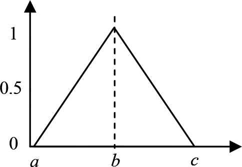
The example of the triangular fuzzy set
4. PROPOSED ALGORITHM
4.1. Solution Representation
Because, the FJSP consists of two sub-problems need to be solved. Therefore, the solution is encoded into two parts. First part represents the sequence of operations and the second part contains the machine which is allocated to each operation in the first part.
In Figure 2, the first part gives the precedence constrained of the operations. The second part presents the machine number which matches to each operation in the first part. The pairing sequence of both parts can be explained as follows.

The example of the solution representation
The first of the number 1 in the operation sequence part represent the first operation of the first job, is to be processed by the machine M3. The first of the number 2 represent the first operation of the second job, is to be processed by the machine M1. The second of the number 1 represent the second operation of the first job, is to be processed by the machine M2. The third of the number 1 represent the third operation of the first job, is to be processed by the machine M2. The second of the number 2 represent the second operation of the second job, is to be processed by the machine M2. The first of the number 3 represent the first operation of the third job, is to be processed by the machine M1 and the second of the number 3 represent the second operation of the third job, is to be processed by the machine M1.
To measure the quality of the solution presented in Figure 2, the makespan is computed as demonstrated in Figure 3.
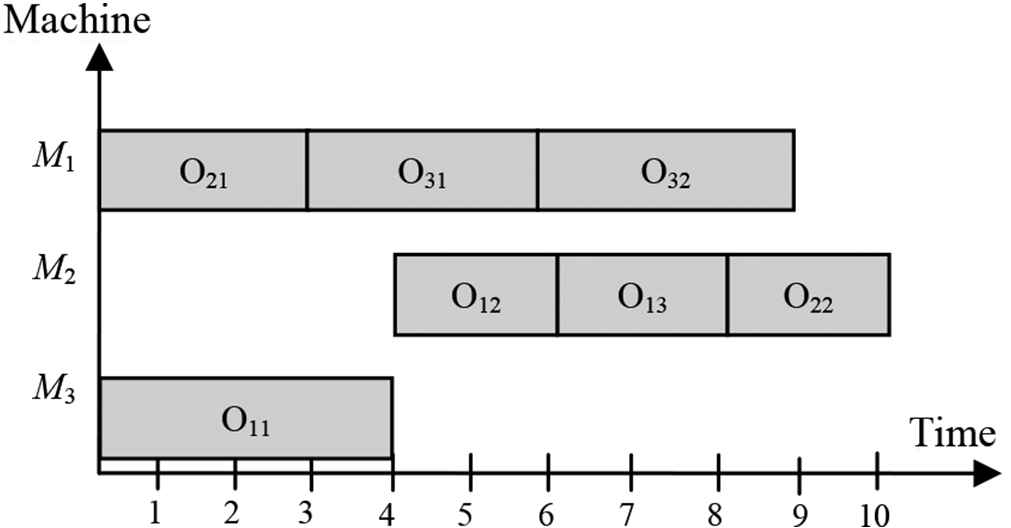
The example of the computation of the makespan
4.2. Generate the Initial Population
The initial population of N solutions is randomly initialized by using a set of the population generation rules as follows:
- •
To create the operation sequence part of the initial population, randomly chosen a number among 1, 2 or 3. When a random number equal to a number 1, the operation sequence part is created by using the random rule. While the random number is 2, the most work remaining rule is used. The most number of operation remaining rules is used when the random number is 3.
- •
This research generates the machine assignment part of the initial population by randomly picked one rule from a set of several rules. This process can be explained step-by-step as follows:
- (a)
Randomly chosen a number between 1 and 2.
- (b)
If the random number equal to 1, using the random rule to produce the machine assignment part. The local minimum processing time rule is used to generate the machine assignment part when the random number is 2.
- (a)
This process repeats until the amount of the initial population is equal to the predefined number.
4.3. Mutation Process
In the proposed algorithm, the mutation process is used as the search mechanism for the promise answer. Because, the solution is divided into two parts. Therefore, the mutation process is split into two stages as follows:
- •
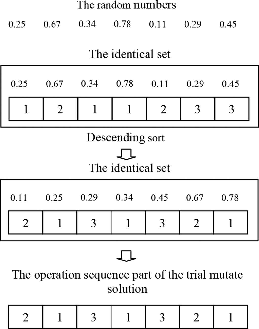
The operation sequence part of the trial mutant solution is produced by applying the arithmetic swapping operation to each of the initial population. The procedure is listed as follows: First, randomly pick the K numbers in the range of 0 and 1. Second, match each of the random number with each operation of the initial population then constructed it into the identical set respectively from left to right. Third, sort the identical set in descending order. At last, defined the identical set as the operation sequence part of the trial mutant solution as indicated in Figure 4.
- •
There are several methods used as the machine selection mechanism such as the operation minimum processing time rule and the random rule. All above methods met the lack of the diversity, as a result, the algorithm is stuck in the local area. Hence, this paper proposed a new idea to choose the proper machine called the fuzzy machine selection. The main concept of the fuzzy machine selection approach is to elect the appropriate machine by considering the machine loads, both the loads of operation number and the loads of machine processing time. In detail, when the machine is overloaded the boundary of fuzzy membership function is small. In contrast, when the machine is independent the size of membership function is large. This gives the available machine higher chance to select. To complete the fuzzy machine selection, the following steps are performed.
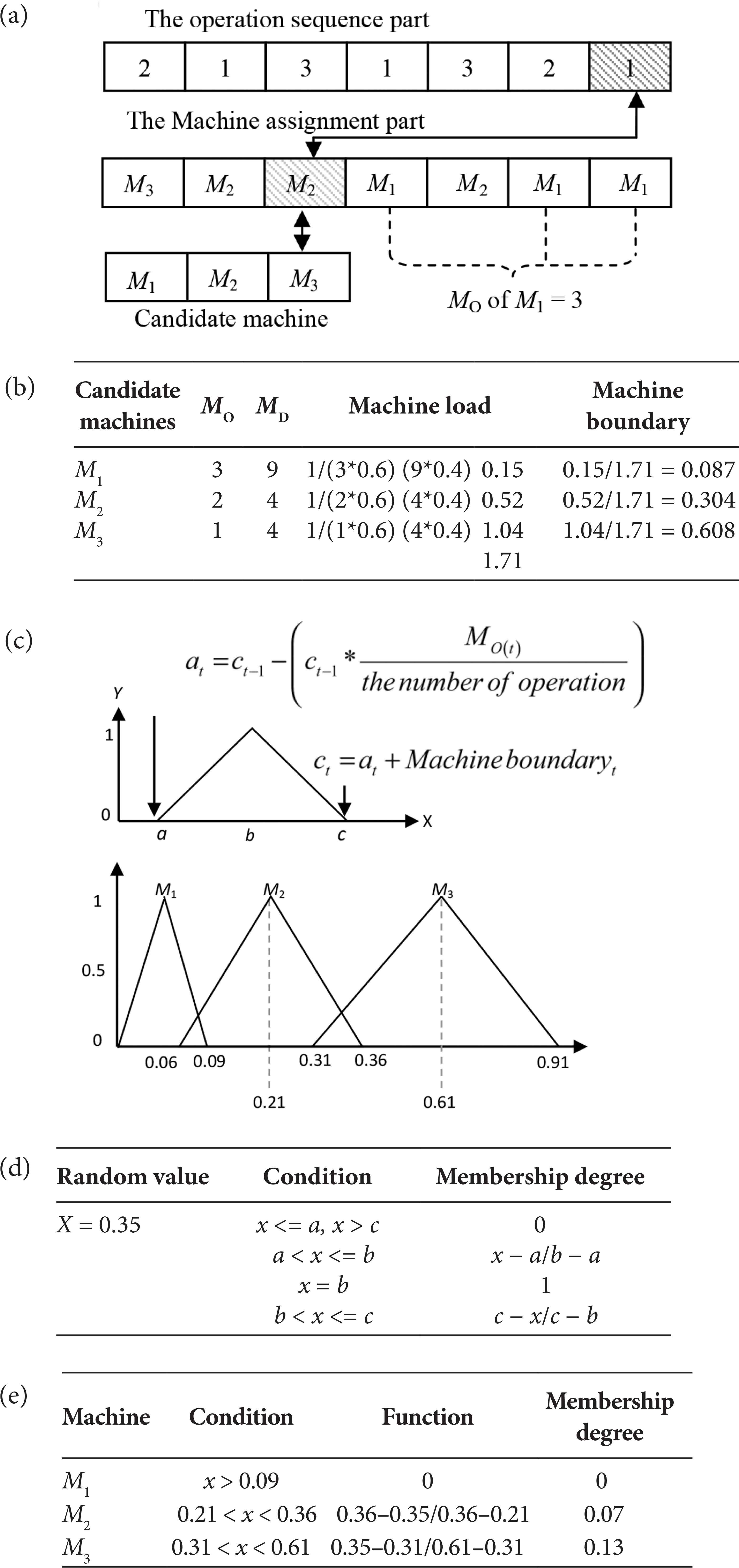
First, we choose one operation in the operation sequence part of the trial mutant solution. After that, record the candidate machine which can assign to the chosen operation as the temporary table. In Figure 5a, the chosen operation is the third operation of the first job.
Second, calculate the loads on each of the candidate machine in the temporary table according to Equation (3), where MO denote the amount of operations loads of each of the candidate machine. MD stated as the accumulated processing time loads of the candidate machine. WO and WD are the defined weight value of MO and MD respectively. The smallest of the Lmi instance appear when the machine heavy load. The computation processes of the candidate machine boundary is shown in Figure 5b.
Third, in Figure 5c, each machine is represented by the triangular membership function. Each of the triangular set represents each of the candidate machines. The size of overlapping between the candidate machine boundaries depends on the load amount of operation. Mean that, if the machine has similar amount of operation loads, then the overlapping size is big.
Fourth, when we created the triangular fuzzy member completely, a random number between 0 and the right corner position of the rightmost membership areas is picked. In Figure 5c, we pick the random number between [0, 0.91].
Fifth, Figure 5d shows the example of the membership degree when a random number is x. The membership degree belongs to each machine is executed according to the triangular membership function which is shown in Figure 5e. The machine with the highest membership degree is selected. This process repeats until the machine assignment part is fulfilled.
The arithmetic swapping operation
The example of the fuzzy machine selection procedure
4.4. Recombination Process
In this process, we randomly match the pair of the trial mutant solutions. After that, the POX crossover and the uniform crossover operation are performed for each pair of solutions to generate the operation sequence part and the machine assignment part of the target solution. The detailed procedure of the POX crossover and the uniform crossover is described as follows:
Figure 6 is an example for the POX crossover operation. To create the operation sequence part of the target solution, the member of the subset is randomly selected. When the subset is completely created, some operation in the trial mutant solution 1 which matched by the member in the subset will transfer to the target solution. At the same time, the rest of the target solution will inherit from the trial mutant solution 2.
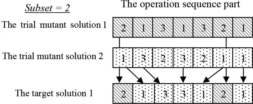
The POX crossover operation
The example of the uniform crossover operation is present in Figure 7. The procedure of this process is started by randomly generating the uniform solution. Then copy the machine of the trial mutant solution 1 that corresponds to the number ‘0’ of the uniform solution to the target solution. The machine of the trial mutant solution 2 that parallel with the number ‘1’ of the uniform solution will copy to the target solution.
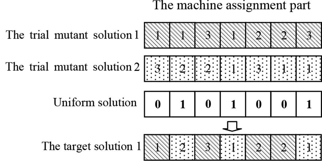
The uniform crossover operation
4.5. Local Search Process
In the proposed algorithm, the local search process is utilized to the best 10% of the target solution. We divided it into two modes. First mode, the best 5% of the target solution is improved by the local search based on the critical path method. Second mode, the remaining 5% is adjusted by the fuzzy machine selection approach. To complete the local search process the following are performed.
- •
The local search based on the critical path method is applied to search for the operation sequence part of the new solution in neighboring areas of the best 5% of the target solution. The critical path is the sequence of the critical operations that defined the duration of the project. It is a longest sequence of the job tasks which must be completed on time to meet the deadline or the minimize duration. When any of the operations in the critical path is late, the project will be delayed. The local search based on the critical path method is proposed to enhance the local exploitation. Mean that, increasing chances of meeting the shorter path. The procedure is explained as follows:
First step: Calculate the critical path as shown in Table 2.
In this table, the column labeled with “Operation sequence” contains the sequence of tasks.
The column label with “Machine” displays the machine number which assigned to each task.
The column label with “Duration” contains the duration time of each task on selected machine.
The column label “Precedence/Operation” show priority in importance of each task. For example, task O21, task O11 and task O31 are performed on the similar machine (M1). Therefore, task O11 can start after task O21 is completed and task O32 can operate after task O11 is finished.
The column label “Precedence/Time” displays the precedence duration related to the “Precedence/Operation” column. The preceding time of the each task is calculated by adding the duration of the preceding operation with the preceding time of the preceding operation. For instance, the preceding operation of O32 has two operations, so, the preceding time has two values.
The value 8 is calculated by adding the duration of task O11 (value 5) with the preceding time (value 3).
The column label “ES” contains the early start time of each task. The early start time is computed by adding the maximum of the preceding time with number 1 [ES = max (precedence time) + 1]. For any task without a predecessor, its early start time will be 1.
The column label “EF” presents the early finish time of the task. This label is calculated by adding the ES with the duration, then subtracting number 1 [EF = (ES + Duration) − 1].
The column label “LF” shows the late finish time, this label is calculated from backward. The last task’s late finish time is same as its early finish time. In addition, the task which last of each job and last of each machine have the late finish time equal to its early finish time. For any task with a single successor, calculate the late finish time by subtracting 1 from its successor’s late start time (LS – 1). Otherwise, calculate its late finish by subtracting 1 from the minimum of its successors.
The column label “LS” displays the late start time of all tasks. The LS is executed by using the following equation: LS = (LF – duration) + 1.
The label “TS” contains the total slack of all tasks. It is calculated by bringing the late start time minus the early start time (LS − ES).
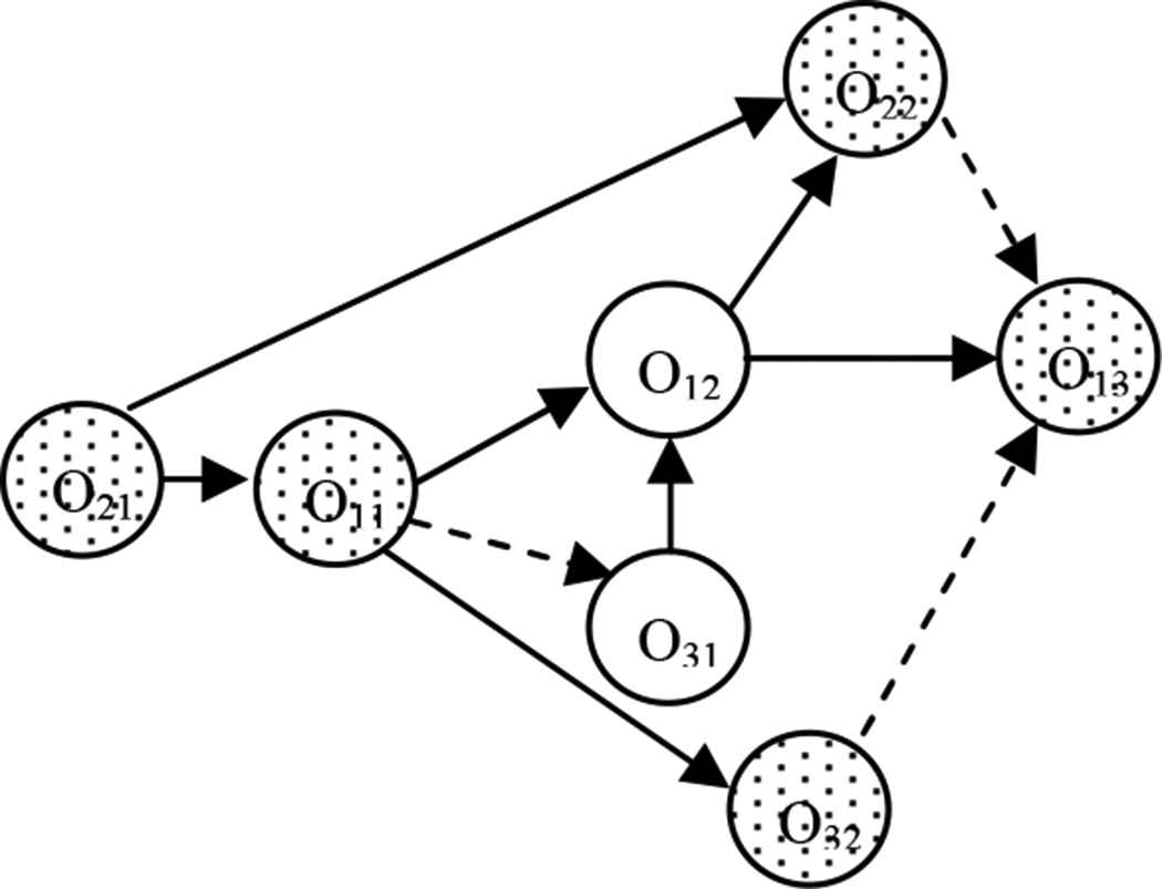
The critical operation is the operation which its total slack equal to 0. In the example, the critical operation is O21, O11, O32, O22 and O13 as shown in Figure 8.
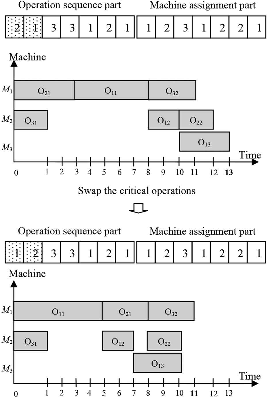
Second step: Move each of the critical operations and insert it at the feasible position. Moving any of the critical operations will obtain the new solution as shown in Figure 9.
Third step: This process repeats until all critical operations moved.
Final step: Replace the target solution by the new solution when the new solution is better.
- •
The fuzzy machine selection is applied to the target solution in the second mode. This mechanism is use to search for the machine assignment part of the new solution. The rationale behind this concept is to enhance the ability to handle the free time of the machine and increase the load balancing among the machines. It is utilized by the following steps.
First step: Calculate to the overall free time of the machine and called as the O time. The O time is the duration which the machine is available. Meanwhile, retrieve to the maximum gap of the free time of each machine and denoted as the GF time. The calculation example of this process is shown in Figure 10.
Second step: Use the fuzzy machine selection to select the machine which proper the free time. According to the procedure of the fuzzy machine selection, the machine which the maximum of the O time and the GF time has a large boundary. Therefore, it has more opportunity to be chosen as shown in Figure 11. We call the machine with the highest membership degree as the available machine.
Third step: Search for the critical operation which the processing time is minimized when assigned to the available machine. Then, assign the above critical operation to the available machine.
Forth step: The new solution will accept when it has a shorter path than the old one.
| Operation sequence | Machine | Duration | Precedence | ES | EF | LS | Successor | LF | TS | ||
|---|---|---|---|---|---|---|---|---|---|---|---|
| Operation | Time | Operation | Time | ||||||||
| O21 | M1 | 3 | – | 0 | 1 | 3 | 1 | O11, O22 | 4, 11 | 3 | 0 |
| O11 | M1 | 5 | O21 | 3 | 4 | 8 | 4 | O32, O12 | 9, 9 | 8 | 0 |
| O31 | M2 | 1 | – | 0 | 1 | 1 | 8 | O32, O12 | 9, 9 | 8 | 7 |
| O32 | M1 | 3 | O11, O31 | 8, 1 | 9 | 11 | 9 | – | – | 11 | 0 |
| O12 | M2 | 2 | O11, O31 | 8, 1 | 9 | 10 | 10 | O22, O13 | 12, 13 | 11 | 1 |
| O22 | M2 | 2 | O21, O12 | 3, 10 | 11 | 12 | 11 | – | – | 12 | 0 |
| O13 | M3 | 3 | O12 | 10 | 11 | 13 | 11 | – | – | 13 | 0 |
The example of the critical path operation calculation
The example of the critical operations
The example of moving the critical operations
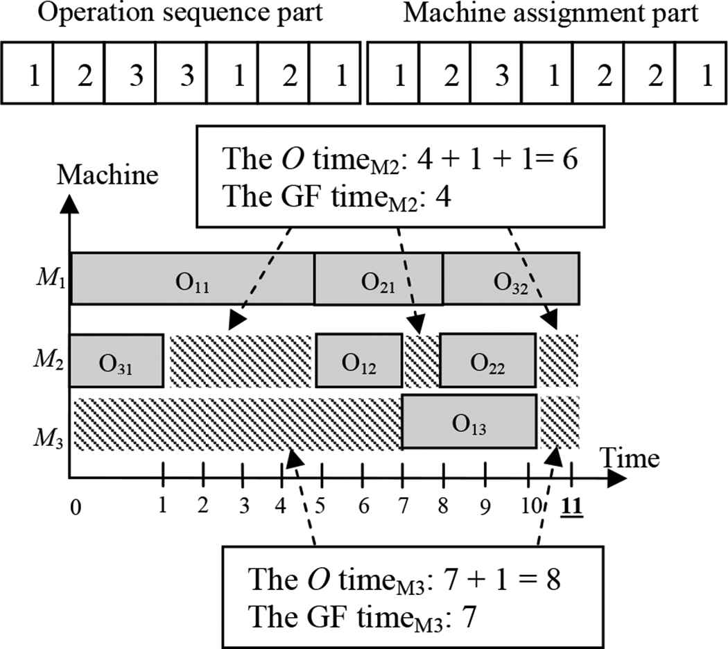
The example of calculating the free time

The example of the membership degree execution
4.6. Selection Process
In the final step, sort all solutions according to the fitness value in descending order. The solutions which their fitness value is in the top N number are defined as the initial population for the next iteration. Then, repeat stage 4.3 through 4.6 until the stopping criteria is met. The proposed algorithm is stopped when the numbers of iteration equal to the predefine number.
5. EXPERIMENTAL RESULTS
To test the performance of the proposed algorithm, the benchmark test sets called the Brandimarte, the Fattahi and the Dauzere Peres Data which obtained from the library of FJSP (FJSPLIB) are used. The effectiveness of the proposed algorithm is compared with the others state-of-the-art algorithm in terms of the average percentage deviation from the lower bound (Avg. Dev. LB (%)).
The Brandimarte data set consists of 10 standard data sets, MK01 to MK10. The MK01 and MK02 consist of 10 jobs with six machines. The MK03 and MK04 contain 15 jobs with eight machines. The MK05 includes 15 jobs with four machines. The MK06 comprises of 10 jobs with fifteen machines. The MK07 consists of 20 jobs with five machines. The MK08–MK10 contain 20 jobs with ten machines.
The Fattahi data set consists of 20 data sets, SFJS1–SFJS10 and MFJS1–MFJS10. Each dataset contains a different number of jobs with distinct a machine number, as follows. The SFJS1 and SFJS2 contain 2 jobs with two machines. The SFJS3–SFJS5 consist of 3 jobs with two machines. The SFJS6–SFJS9 include 3 jobs with three, five, four and three machines respectively. The SFJS10 contains 4 jobs with five machines. The MFJS1–MFJS7 include seven machines with 5, 5, 6, 7, 7, 8 and 8 jobs respectively. The MFJS8–MFJS10 contain eight machines with 9, 11 and 12 jobs respectively.
The Dauzere Peres and Paulli data set contains 18 standard data sets named 01a–18a. The 01a–06a consist of 10 jobs with five machines. The 07a–12a provide 15 jobs with eight machines. The last, 13a–18a include 20 jobs with ten machines.
Tables 3–5 illustrates the comparative results of the proposed algorithm with the three related algorithms. The column labeled with “LB” displays the minimum boundary of each problem data set. The followings are present the comparative results.
| Problem | LB | Proposed algorithm | QPSO [11] | SSPR [12] | HDE [13] |
|---|---|---|---|---|---|
| MK01 | 36 | 39 | 37 | 40 | 40 |
| MK02 | 24 | 26 | 26 | 26 | 26 |
| MK03 | 204 | 204 | 204 | 204 | 204 |
| MK04 | 48 | 59 | 60 | 60 | 60 |
| MK05 | 168 | 172 | 173 | 172 | 172 |
| MK06 | 33 | 57 | 64 | 57 | 57 |
| MK07 | 133 | 139 | 139 | 139 | 139 |
| MK08 | 523 | 523 | 523 | 523 | 523 |
| MK09 | 299 | 307 | 307 | 307 | 307 |
| MK10 | 165 | 197 | 205 | 196 | 198 |
| Avg. Dev. LB (%) | 14.127 | 16.446 | 14.553 | 14.674 | |
The comparative result of the Brandimarte data
| Problem | LB | Proposed algorithm | AIA [14] | AISA [15] | SA [16] |
|---|---|---|---|---|---|
| SFJS1 | 66 | 66 | 66 | 66 | 66 |
| SFJS2 | 107 | 107 | 107 | 107 | 107 |
| SFJS3 | 221 | 221 | 221 | 221 | 221 |
| SFJS4 | 355 | 355 | 355 | 355 | 355 |
| SFJS5 | 119 | 119 | 119 | 119 | 119 |
| SFJS6 | 320 | 320 | 320 | 320 | 320 |
| SFJS7 | 397 | 397 | 397 | 397 | 397 |
| SFJS8 | 253 | 253 | 253 | 253 | 253 |
| SFJS9 | 210 | 210 | 210 | 210 | 210 |
| SFJS10 | 516 | 516 | 516 | 516 | 516 |
| MFJS1 | 396 | 468 | 468 | 468 | 468 |
| MFJS2 | 396 | 446 | 448 | 446 | 448 |
| MFJS3 | 396 | 466 | 468 | 466 | 468 |
| MFJS4 | 496 | 554 | 554 | 554 | 561 |
| MFJS5 | 414 | 514 | 527 | 514 | 514 |
| MFJS6 | 469 | 608 | 635 | 608 | 634 |
| MFJS7 | 619 | 879 | 879 | 879 | 899 |
| MFJS8 | 619 | 884 | 884 | 894 | 897 |
| MFJS9 | 764 | 1055 | 1088 | 1088 | 1101 |
| MFJS10 | 944 | 1201 | 1267 | 1196 | 1258 |
| Avg. Dev. LB (%) | 13.205 | 14.27 | 13.475 | 14.473 | |
The comparative result of the Fattahi data
| Problem | LB | Proposed algorithm | QPSO [11] | SSPR [12] | HHS/LNS [17] |
|---|---|---|---|---|---|
| 01a | 2505 | 2505 | 2505 | 2505 | 2505 |
| 02a | 2228 | 2230 | 2230 | 2229 | 2230 |
| 03a | 2228 | 2228 | 2229 | 2228 | 2228 |
| 04a | 2503 | 2503 | 2498 | 2503 | 2506 |
| 05a | 2189 | 2211 | 2207 | 2211 | 2212 |
| 06a | 2162 | 2180 | 2170 | 2183 | 2187 |
| 07a | 2187 | 2220 | 2264 | 2274 | 2288 |
| 08a | 2061 | 2066 | 2073 | 2064 | 2067 |
| 09a | 2061 | 2064 | 2066 | 2062 | 2069 |
| 10a | 2178 | 2210 | 2205 | 2269 | 2297 |
| 11a | 2017 | 2058 | 2050 | 2051 | 2061 |
| 12a | 1969 | 2020 | 2019 | 2018 | 2027 |
| 13a | 2161 | 2198 | 2253 | 2248 | 2263 |
| 14a | 2161 | 2163 | 2167 | 2163 | 2164 |
| 15a | 2161 | 2153 | 2165 | 2162 | 2163 |
| 16a | 2148 | 2213 | 2252 | 2244 | 2259 |
| 17a | 2088 | 2130 | 2134 | 2130 | 2137 |
| 18a | 2057 | 2123 | 2123 | 2119 | 2124 |
| Avg. Dev. LB (%) | 1.089 | 1.437 | 1.567 | 1.890 | |
The comparative result of the Dauzere Peres and Paulli data
In Table 3, the Brandimarte data set, all comparison algorithms successfully found the optimum results of MK03 and MK08. For MK02, MK05, MK07–MK09, the proposed algorithm, the SSPR and the HDE reach the best path. In MK06, the proposed algorithm, the SSPR and the HDE met the best answer. The MK04, the proposed algorithm is outperforming. The QPSO comes in first place with MK01 and followed by the proposed algorithm. Likewise the MK10, the SSPR comes in first place and a second place is the proposed algorithm. When considering all instances together, our proposed algorithm found solutions that nearest lower bounds, at 14.127% mean relative error.
Table 4, the fattahi data set, shows that all algorithms accomplished found the best result of SFJS1 through MFJS1. For MFJS2–MFJS6, the proposed algorithm and the AISA obtain the best of minimum results. The proposed algorithm, the AIA and the AISA come for first place for MFJS7. For the MFJS8 problem, the proposed algorithm and the AIA met the best answer and followed by the AISA. The proposed algorithm outperforms than the other comparison algorithm with the hardest data set MFJS9 and MFJS10. When looking at all datasets together found that, the average percentage deviation from the lower bound of the proposed algorithm is the most performance among the comparison algorithm at 13.205% mean relative error.
Table 5 illustrates the comparative result of the proposed algorithm and the current state-of-the-art meta-heuristic algorithms tested with the Dauzere Peres and Paulli data set. For 01a, all comparison algorithms achieved the best results. For 02a, the SSPR met the best result followed by the other comparison. For 03a, the proposed algorithm is in line with the SSPR and the HHS/LNS. The proposed algorithm and the SSPR met the best result of the 04a, 05a, 14a and 17a. The QPSO founded the best minimum answer of the 06a and 10a and followed by the proposed algorithm. For 07a, 13a, 15a and 16a the proposed algorithm has the smallest difference when compared with the LB answer. For 08a, 09a and 18a, the SSPR comes in first place and followed by the proposed algorithm. For the 11a and 12a problem, the QPSO and the SSPR contain the best result and the proposed algorithm comes in second place. As the Avg. Dev. LB (%) results, the proposed algorithm is the best competitor.
6. CONCLUSION
This paper presents the new algorithm which is based on the step of DE algorithm. In the proposed algorithm, the new mechanism called the fuzzy machine selection is presented to create the machine membership function used to select the proper machine. In the mutation process, the arithmetic swap operation and the fuzzy machine selection mechanism embedded the loads balancing criteria is used. Then, the local search based on the critical path method and the fuzzy machine selection embedded the free time criteria are utilized in the local search process. The proposed algorithm is tested with 48 datasets. The result indicates that the proposed algorithm is outperforming than the other comparison algorithms.
REFERENCES
Cite this article
TY  - JOUR
AU  - Ajchara Phu-ang
PY  - 2018
DA  - 2018/12/31
TI  - Discrete Differential Evolution Algorithm with the Fuzzy Machine Selection for Solving the Flexible Job Shop Scheduling Problem
JO  - International Journal of Networked and Distributed Computing
SP  - 11
EP  - 19
VL  - 7
IS  - 1
SN  - 2211-7946
UR  - https://doi.org/10.2991/ijndc.2018.7.1.2
DO  - 10.2991/ijndc.2018.7.1.2
ID  - Phu-ang2018
ER  -