
Automatic clustering based on Crow Search Algorithm-Kmeans (CSA-Kmeans) and Data Envelopment Analysis (DEA)
- DOI
- 10.2991/ijcis.11.1.98How to use a DOI?
- Keywords
- Automatic Clustering; K-Means; Crow Search Optimization Algorithm; Cluster Validity Indices; Data Envelopment Analysis
- Abstract
Cluster Validity Indices (CVI) evaluate the efficiency of a clustering algorithm and Data Envelopment Analysis (DEA) evaluate the efficiency of Decision-Making Units (DMUs) using a number of inputs data and outputs data. Combination of the CVI and DEA inspired the development of a new automatic clustering algorithm called Automatic Clustering Based on Data Envelopment Analysis (ACDEA). ACDEA is able to determine the optimal number of clusters in four main steps. In the first step, a new clustering algorithm called CSA-Kmeans is introduced. In this algorithm, clustering is performed by the Crow Search Algorithm (CSA), in which the K-means algorithm generates the initial centers of the clusters. In the second step, the clustering of data is performed from kmin cluster to kmax cluster, using CSA-Kmeans. At each iteration of clustering, using correct data labels, Within-Group Scatter (WGS) index, Between-Group Scatter (BGS) index, Dunn Index (DI), the Calinski-Harabasz (CH) index, and the Silhouette index (SI) are extracted and stored, which ultimately these indices make a matrix that the columns of this matrix indicate the values of validity indices and the rows or DMUs represent the number of clustering times from kmin cluster to kmax cluster. In the third step, the efficiency of the DMUs is calculated using the DEA method based on the second stage matrix, and given that the DI, CH, and SI estimate the relationship within group scatter and between group scatter, WGS and BGS are used as input variables and the indices of DI, CH and SI are used as output variables to DEA. Finally, in step four, AP method is used to calculate the efficiency of DMUs, so that an efficiency value is obtained for each DMU that maximum efficiency represents the optimal number of clusters. In this study, three categories of data are used to measure the efficiency of the ACDEA algorithm. Also, the efficiency of ACDEA is compared with the DCPSO, GCUK and ACDE algorithms. According to the results, there is a positive significant relationship between input CVI and output CVI in data envelopment analysis, and the optimal number of clusters is achieved for many cases.
- Copyright
- © 2018, the Authors. Published by Atlantis Press.
- Open Access
- This is an open access article under the CC BY-NC license (http://creativecommons.org/licences/by-nc/4.0/).
1. Introduction
The clustering problem is an unsupervised technique, which, by processing data in the feature space makes similar samples to be placed in separate clusters. The clustering technique is widely used in image segmentation, data compression, pattern recognition, and machine learning 1. In general, the algorithms used in clustering methods are divided into two categories: hierarchical and partitioning 2–4. These algorithms consider two factors for clustering, including cohesion and separation. In cohesion, similarity within a cluster is calculated and in separation, the dissimilarity between clusters is calculated. Many algorithms perform clustering given a predetermined number of clusters without determining the optimal number of clusters. For some data, it is difficult to determine the optimal number of clusters, especially when the number of dimensions increases or when data is compressed which is considered as one of the major weaknesses. At the end of 1990, the automatic clustering was investigated as a new method in cluster analysis to overcome this weakness. The main objective of automatic clustering is to determine the optimal number of clusters automatically. Different methods have been proposed to determine the optimal number of clusters, which solving the automatic clustering problem with the help of metaheuristics algorithms is more pronounced. These algorithms are divided into three groups of single-solution-based, population-base, and multi-objective algorithms. Population-based algorithms are also divided into three groups of evolutionary algorithms, swarm intelligence algorithms, and Artificial Immune Systems algorithms. One of the major methods for the automatic determination of the optimal number of clusters automatically is a combination of swarm intelligence algorithms with Cluster validity indices (CVI) 5 as an objective function. CVI measure the efficiency of a clustering algorithm using intrinsic data, and usually, these indicators estimate the relationship between intra-cluster scattering and scattering between clusters in order to examine the quality of clustering algorithms 6.
In this study, a new algorithm called Automatic Clustering Based on Data Envelopment Analysis (ACDEA) is presented which can determine the optimal number of clusters. The main idea of this algorithm is to use a combination of CVI and Data Envelopment Analysis (DEA). DEA is one of the best efficiency analysis techniques. This method was first proposed by Charens et al. 7, which can evaluate the efficiency of different Decision-Making Units (DMUs). The selection of input and output variables is one of the most important steps in modeling using DEA. In this study, CVI are considered as input and output variables and the number of clusters as DMUs. The difference between this method and previous works is that the CVI are analyzed simultaneously using the DEA and the efficiency of each clustering is measured. In addition, the Crow Search Algorithm (CSA) 8 is used for the clustering in which the initial centers of the clusters are generated by the K-Means algorithm, which is called the CSA-Kmeans algorithm.
In the following, after reviewing the literature, in the third section, five cluster validity indices of Within-Group scatter (WGS) 9, Between-Group scatter (BGS) 5, Dunn Index (DI) 10, Calinski-Harabasz (CH) index 11 and the Silhouette Index (SI) 12 are described. In the fourth section, the CSA-Kmeans clustering algorithm and the steps of ACDEA algorithm will be described. The results of using ACDEA algorithm are presented in three different types of data, and its efficiency is compared with the DCPSO 13, ACDE 14, CGUK 15 algorithms in section five, and finally, in section six, the conclusion is presented.
2. Related works
population-based metaheuristics have shown better efficiency in the field of automatic clustering and most automatic clustering algorithms are based on these algorithms 3. A group of population-based algorithms are swarm intelligence-based algorithms known as SI 16. In these algorithms, there is a direct and indirect relationship between different solutions and are inspired by the swarm behaviors of animals, insects and other living things in nature. One of the most widely used SI algorithms is the PSO algorithm 17. This algorithm is one of the most popular SI algorithms, and automated clustering approaches based on this algorithm include: DCPSO 13, MEPSO 18, PSOPS 19, DCPG 20. In the DCPSO algorithm, the optimal number of clusters is obtained by the PSO algorithm and the centers are achieved by the k-means algorithm. Also, the indices of DI, Turi Index (TI) 21 and S_Dbw index 22 are used as the objective function. In the MEPSO algorithm, the cluster centers and activation threshold are used to encoding the solution, and the Xie-Beni (XB) index 23 is used as the objective function that determines the active and inactive clusters. In the PSOPS algorithm, cluster centers are used to encoding the solution and the Sym-index 24 is used as the objective function. In the DCPG hybrid algorithm, GA 25 and PSO algorithms are used for clustering and the TI index as an objective function. Ant Colony Optimization (ACO) 26 algorithm, Bee Colony Optimization (BCO) 27 algorithm and Invasive Weed Algorithm (IWO) 28 were also used for automatic clustering. The ant-clustering 29, ATTA-C 30, were formed based on the ACO, AKC-BCO 31 was formed based on the BCO, and the IWO-clustering algorithm 32 was formed based on the IWO algorithm. The ATTA-C algorithm uses the fuzzy c-means algorithm 33 as the initial phase, and then the optimal number of clusters is determined using the ACO. Here, the neighborhood function (NF) is used as the objective function. The AKC-BCO algorithm uses the cluster centers and the activation threshold to encode the solution, and the Gaussian kernel and the CS index 34 are used as the objective function. IWO-clustering algorithm uses cluster centers in order to encode the solution and afford from the modified sym-index as the objective function.
3. Background
CVI, measure the efficiency of a clustering algorithm using clustered data. In following some related basic definitions will be explained.
3.1. Basic Definitions
An object is considered as a data and defined by the vector x = {x1, x2, …, xD}T, where xi ∈ ℝ and D represent the dimensions. X = {x
1
, x
2
, …, x
N
} represents a dataset with N object. A cluster is a set of massive data that is scattered in the feature space and the segmentation of the dataset X into a discrete k group is called clustering C
= {ck|k = 1, …, K}. The cluster center of ck is defined as
3.1.1. Cluster Validity Indices
Within-Group Scatter index (WGS): This indicator measures the square of the distance between the points within a cluster and the center of the cluster which is defined by Eq. (1):
Between-Group Scatter index (BGS): This index measures the total distance between two clusters which is formulated based on Eq. (2):
Dunn Index (DI): This index has different types and is considered as a ratio-type index whose basic formula is defined according to Eq. (3):
Where
According to Eq. (3), the cohesion is calculated using the nearest neighbor method and separation is estimated by using the maximum diameter of the clusters. δ represents the within-cluster distance and Δ represents the between-cluster distance.
Calinski-Harabasz index (CH): This index is used for the crisp clustering algorithms so that it mathematical model is based on Eq. (4):
In Eq. (4), cohesion is calculated by the sum of distances between points of the cluster from the global center of the cluster and separation is calculated by the sum of the distances of each cluster center with the global center of the dataset.
Silhouette index (SI): This index is considered as a normalized summation type index, whose equation is defined as follows:
Where
Based on Eq. (5), in order to calculate the cohesion, the sum of the distances between all points in the same cluster is calculated and separation is estimated by the nearest neighbor distance between points in different groups.
4. The proposed algorithm
When data is compressed or data dimension increase, it is possible that the results of the CVI will lead to clustering algorithms show different performance in determining the optimal number of clusters, which is considered as one of the major weaknesses. This is because of the difference in how you calculate the amount of within-cluster scatter and between-cluster scatter. For example, DI use the nearest neighbor method to calculate cohesion and the maximum cluster diameter method to calculate the separation while SI uses the sum of the distances between all the points in the same cluster to calculate the cohesion and the nearest neighbor distance between points in different groups to calculate the separation. To reduce this weakness, in this study, the ACDEA algorithm is proposed. This algorithm, that combines CVI and DEA, seeks to determine the optimal number of clusters and provide better results than other CVI and clustering algorithms. Based on the pseudocode of Fig. 1, four main steps can be defined in the design of this algorithm, so that after inputting data, the process of determining the optimal number of the clusters can be formed by these steps: Clustering by the CSA-Kmeans algorithm 2- Extraction and storing CVI by running CSA-Kmeans algorithm based on kmin cluster to kmax cluster 3. Ranking of DMUs using input-oriented CCR method. 4. Ranking of efficient DMUs using AP method and reporting the best number of clusters. So, there are three new features in this algorithm that distinguish it from other algorithms. These features are 1. Use of the new combination of CSA and K-means for clustering. 2. Simultaneous use of cumulative CVI. 3. Use of DEA to verify the efficiency of clusters. In the following, the steps related to Fig. 1 will be discussed.
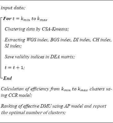
Pseudocode of the ACDEA
4.1. Input data
Combined data is widely used to examine the efficiency of automatic clustering algorithms. Researchers have often used combination data and real datasets to compare the efficiency of different algorithms. In this study, three categories of data are used. The first and second groups include combined data and the third category includes real data. Features such as the number of clusters, number of data records, degree of data overlap, the dimension and the data form are considered as the criteria for categorizing data in different groups. The first category data includes data with less cluster number and lower degree of overlap, and the second group contains data with more number of clusters and overlap. The actual data is placed in the third category, which has more dimensions and different forms.
4.2. Clustering by the CSA-Kmeans algorithm
The Crow Search Algorithm (CSA) is considered as one of the recent algorithms introduced in the field of swarm intelligence. This is very simple algorithm inspired by the social behavior of the crow. The main idea behind this algorithm is to find the secret places of the crows in order to find food and steal from each other. In such a way that, when the crow j plans to visit its secret place, the crow i decides to follow the crow j. In this situation, two conditions occur: in the first state, the crow j does not know about the existence of a crow i, and the crow i moves towards the secret place of the crow j. In the latter state, the crow j is aware of crow i and in order to protect its storage will direct crow i to an unspecified place. New solutions are generated based on this structure, and different parts of the solution space are searched in successive iteration to reach the optimal solution or close to optimal solution.
The K-Means algorithm is one of the most common clustering methods, which, despite many advantages, including high speed and ease of implementation, is trapped into local optima and does not always generate the optimal solution. On the other hand, metaheuristic algorithms are also able to cluster data with random and heuristic logics, but do not necessarily guarantee the generation of the optimal solution of clustering. So, CSA is used for clustering to create a high probability of convergence to optimal solution, with this aid that the initial centers of the clusters are generated using the K-Means algorithm. This combination is called CSA-Kmeans that can lead to leaving local minima and generate the optimal solution of the problem with a high percentage.
Given that the use of an appropriate objective function in the metaheuristic algorithms can have a significant effect on the quality of clustering, the CS index is also used as the objective function which was introduced by Chou et al. 34. The CS index is defined by the Eq. (6):
Where
The CS index is considered as a ratio-type index, which calculates the ratio of cohesion to the separation. The measure related to the calculation of cohesion is the measurement of the clusters diameter and separation calculation is the measurement of the distance of the nearest neighbor between clusters centers. Based on Eq. (7), CSi is the CS index, which evaluated on the ith solution for CSA. Given that the lower value of the CS index represents a clustering with better quality, the formula
Several methods have been proposed to measure the distances between data in the clustering problem. Therefore it is necessary that a proper method to be selected in order to measure the distances because the selection of each of these distances can create different groups in clustering 35. Among the methods presented for measuring distances, the Minkowski metric 36 is widely used to solve the automatic clustering problems. In this study, the Minkowski metric is used for measuring the distances, which its formula is based on Eq. (8):
It should be noted that, for p = 1, the city block37, for p = 2, Euclidean metric and for p = ∞, Chebyshev metric38 is calculated.
The summary of the CSA-Kmeans algorithm is shown in Fig. 2. Based on this pseudocode, after inputting data and the number of clusters, using the K-means algorithm, the cluster centers are created according to the initial population of the crows, which each member has k cluster centers, which represents the fixed-length encoding structure. Then, these centers are evaluated by the CS index, and the value of the objective function is extracted with the data labels. After initial memory preparation, the algorithm enters the main phase, which has two main loops. In the inner loop, a vector of cluster center is randomly selected from the main population, and then after initializing variable AP, two states are created:
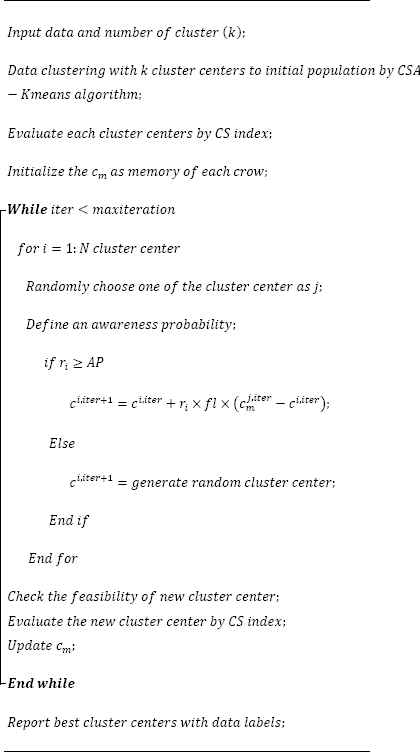
Clustering by CSA-Kmeans
State 1: In the ith iteration, the value of ri is generated randomly between zero and one, and if ri ≥ AP, the ith centers (ci,iter) move towards the jth centers (
State 2: If ri < AP, the new center will be generated randomly.
In the following, acceptable solutions (solutions that are located within lower and upper bound of solution space) are investigated and the new values of the centers are evaluated by the CS index and the value of the variable cm is updated using acceptable solutions. This process continues until it reaches the stopping criteria (maximum iteration value) and the completion of the outer loop. Finally, the best cluster centers are reported by this algorithm with the correct data label.
4.3. Extracting Validity indices
As shown in Fig. 3, at the end of each stage of clustering using the CSA-Kmeans algorithm, clustering, centers, and the correct data label are extracted as clustering output. These outputs are considered as inputs for calculating the values of CVI. In this study, five validity indices have been used, which include: WGS, BGS, DI, CH, and SI. The results of each CVI indicate the quality and efficiency of the clustering. The highest values in the BGS, CH, DI, and SI and the smallest value in the WGS, represent the optimal cluster number. Based on Fig. 4, in this method, we will have a matrix with n columns and m rows, where columns represent the values of CVI and the number of rows is kmax − kmin, that is in the first iteration, data clustering is done with kmin number of clusters, in the second iteration, data clustering is performed based on the kmin + 1 clusters, and finally, in the last iteration, the data clustering is performed based on the kmax number of cluster. At each stage, the values of the validity indices are saved and after reaching kmax, CVI matrix are generated. Im, n, in Fig 4 represents the value of the nth index when the clustering is performed with m cluster. For example, I2,1 represents value of the first index when clustering is performed with two clusters. In order to calculate CVI, at least two clusters are required. So, always kmin ≥ 2 is held.
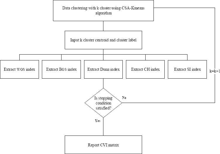
Flowchart of extracting CVI
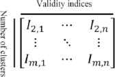
The matrix of CVI as input to DEA
4.4. Formation of input matrix for DEA
A number of inputs and outputs are defined to measure efficiency in the DEA method. In the proposed algorithm, inputs and outputs are determined based on the value of CVI that the correct selection of these indices can help to better differentiate the efficiency of the DMUs. Given that the relationship between input indices and output indices is one of the main assumptions in data envelopment analysis, therefore WGS and BGS can be considered as input values, and the DI, CH, and the SI can be considered as output indices, because DI, CH, and SI estimate the relationship between within-cluster scatter and the difference between clusters in order to estimate the quality of the clustering 6, which means that the values of output indices are created with receiving input values. It has been proven that in order to obtain usable and analytic efficiency, always S ≥ 3 (I + O), where I is the number of inputs, O is the number of outputs, and S is the number of DMUs. Accordingly, I include WGS and BGS, and O contains the DI, CH, and SI. Given that there are 2 inputs and 3 outputs, we should have S ≥ 15. Accordingly, in order to obtain a usable efficiency, always clustering operations are carried out from 2 clusters to 17 clusters. kmax is used as stopping criterion for the number of clusters. Therefore, after reaching the number 17, clustering is stopped and after making the CVI matrix, it is used to calculate the efficiencies and determine the best number of the cluster in the next stage.
4.5. Calculation of efficiency using the input-oriented CCR model
DEA is Farrell’s Idea Development in relation with the calculation of efficiency using the production function. 20 years after Farrell’s outstanding work, Charnes, Coopers, and Rhodes, developed a creative approach on the basis of previous works, which is known as the CCR model to calculate the relative efficiency of DMUs. In CCR model, each unit is known as DMU, and input and output must be non-negative numbers. The objective function and constraints of the CCR model are based on the (10):
Subject to:
Where θj is the efficiency of jth unit (0 ≤ θj ≤ 1 ), uk is the weight of the kth output (k = 1, …, s), ve is the weight of the eth input (e = 1, …, m), Okj is the amount of the kth output in the jth DMU, Iej is the amount of the eth input in the jth DMU. This optimization problem can be formulated in a linearized form based on (11):
Subject to:
The aim of this model is to find the maximum output in DMUp with respect to input constraints, which are known as the Linear Input-Oriented Model. The aim of the DEA models with the input-oriented approach is to achieve a technical inefficiency ratio that should be reduced in inputs so that the DMU remains in the efficiency boundary without changing the output. But the aim of the output-oriented view is to find a ratio that should increase outputs so that the DMU can reach efficiency boundary without changing inputs.
In order to model our problem based on the CCR model, suppose that DMUj (j = kmin, …, kmax, ) be a DMU related to a feasible clustering with j number of clusters which yields DMU’s inputs and outputs such that for each j:
xj = (x1j, …, xmj) is the input vector and yj = (y1j, …, ysj) is the vector of output values for the DMUj. Given that two CVI are used as inputs, therefore xj= (x1j, x2j), where x1j represents the value of the WGS and x2j is the value of the BGS in DMUj. Also, yj = (y1j, y2j, y3j) where y1j represents the value of the CH, y2j, the value of the DI, and y3j is the value of SI in the DMUj. Therefore, the linearized form of the CCR model can be shown as (12):
Subject to:
According to the flowchart of Fig. 5, after the input CVI matrix and using CCR technique, an efficiency value is obtained for each DMU, which ultimately the highest efficiency indicates the most efficient DMU or the optimal number of the cluster. For example, if the efficiency of the fourth DMU is maximized, it indicates that there are suitable four clusters fitted to data. In some cases, due to the type of data, there is more than one cluster with maximum efficiency. CCR basic models do not allow comparisons between efficient DMUs due to the lack of full ranking between the efficient DMUs. In other words, this model divides the DMUs under study into two groups of efficient DMUs and inefficient DMUs. Inefficient DMUs can be ranked by obtaining an efficiency score, but efficient DMUs cannot be ranked because they have the same efficiency score (DMU efficiency). Therefore, some researchers have suggested ways to rank these efficient DMUs, among which the Andersen and Peterson model (AP) is one of the most famous one 39. This method is classified in Super efficiency category and its general form is based on (13):
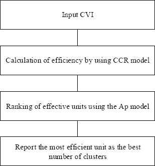
Determining the best number of clusters using CCR and AP method
Subject to:
Based on model (13), in the AP method, the corresponding constraint of the DMU is removed from the evaluation. This constraint causes the maximum value of the efficiency to be one. The efficiency of DMU by eliminating this constraint can be more than one, which provides the ability to compare efficient DMUs. In (14), our problem is modeled based on the AP method. According to the AP method, DMU that has the highest efficiency level is known as the most efficient DMU that determines the best number of clusters.
Subject to:
5. Evaluation of the proposed algorithm
In this section, three sets of test data are used to evaluate the efficiency of the ACDEA algorithm. Table 1 shows a summary of the data, along with the number of data points per data, and the optimal number of clusters. According to this table, the first category includes test data from D2 to D9, the second category includes testing data from S1 to S4. There are also a number of real datasets including Iris, Wine, Breast-Cancer, Vowel, which are laced in the third group. The efficiency of the ACDEA algorithm is compared with other algorithms on real datasets. At the end of this section, the values of CVI along with efficiency levels are presented for real datasets.
| Group of data | Dataset | Number of data point | The optimal number of clusters |
|---|---|---|---|
| First group of data | D2 | 200 | 2 |
| D3 | 250 | 3 | |
| D4 | 400 | 4 | |
| D5 | 500 | 5 | |
| D6 | 600 | 6 | |
| D7 | 650 | 7 | |
| D8 | 800 | 8 | |
| D9 | 1800 | 9 | |
| D10 | 2000 | 10 | |
| Second group of data | S1 | 5000 | 15 |
| S2 | 5000 | 15 | |
| S3 | 5000 | 15 | |
| S4 | 5000 | 15 | |
| Iris | 150 | 3 | |
| Third group of data | Wine | 178 | 3 |
| Breast-Cancer | 699 | 2 | |
| Vowel | 5687 | 6 | |
Test datasets
5.1. First group of data
This group contains dataset D2 to D9 in two dimensions. These data are clustered using the CSA-Kmeans algorithm. The clustered schematic of these data are shown in Fig. 6. In this figure, each cluster is represented by a distinct color, and the number of clusters is optimal. Datasets D2 to D9 have hyper-spherical and hyper-elliptic clusters. As an example, in D9, a number of clusters are hyper-spherical and a number of clusters are hyper-elliptic. The graphs in Fig. 7 shows the efficiency achieved for DMUs or the associated number of clusters. The maximum peak in these graphs represent the most efficient DMU, or in other words, represents the optimal number of clusters. In Fig. 7, clustering is performed on data D2 from two clusters to 17 clusters. This figure shows that the proper number of clusters for this dataset is two and nine while twelve clusters may also be suitable, while the efficiency of these clusters is higher than one and the most efficient cluster is specified using the AP method. Accordingly, in part b, three clusters are suitable for data D3, in part c, four clusters for data D4, in part c, five clusters for data D5, in part e, six clusters for data D6, in part f, seven clusters for data D7, in part g, eight clusters for data D8, in part h, nine clusters for data D9, and in part i, 10 clusters for data D10. The results in Fig. 7 show that for all of datasets in the first group of data, the ACDEA algorithm has an optimum performance and determines the optimal number of clusters. In general, the ACDEA algorithm can be considered as an efficient algorithm to identify the optimal number of clusters for data with hyper-spherical and hyper-elliptic clusters.
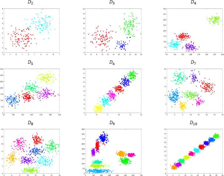
Data plot for D2 to D10
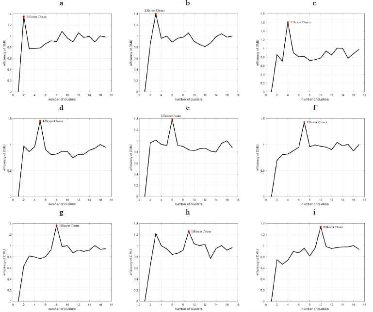
Efficiency of clusters for D2 to D10
5.2. Second group of data
This set of data includes the synthetic data S1–S4 that have two dimensions, and each of datasets has a variable complexity and different overlapping degrees 40. Fig. 8 shows the scatter plot of these data. According to this figure, there are 15 optimal clusters for each dataset. According to the results obtained in Fig. 9, for all datasets S1 to S4, the ACDEA algorithm shows the maximum efficiency at 15 clusters and has reached the optimal solution. Fig. 9 shows that for S1 and S2, only the case with15 number of clusters has the efficiency of one; for S3, 15 and 16 number of clusters have the efficiency of greater than one, where the case of 15 clusters has a higher efficiency which is relevant to the best number of clusters. for S4, there are 14, 15, and 16 clusters have the efficiency greater than one, which ultimately 15 clusters are proposed as the most efficient cluster number. In total, it can be concluded that with an increase in the overlapping of clusters, the optimal number of clusters can be determined by ACDEA method.
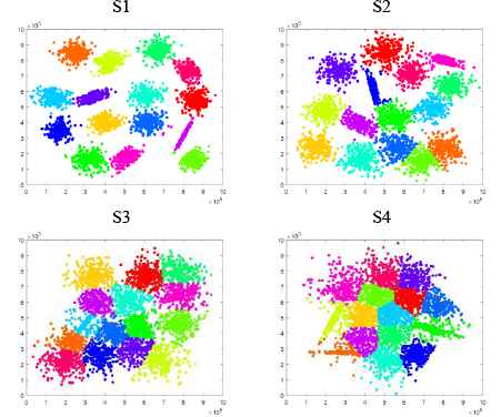
Synthetic 2-d data with N=5000 vectors and k=15 Gaussian clusters with different degree of cluster overlapping
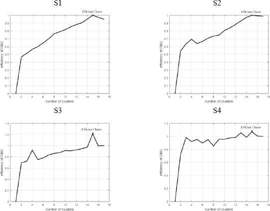
Efficiency of clusters for S1 to S4
5.3. Third group of data
The real data in the clustering field can be used as an appropriate source to investigate the efficiency of the various clustering algorithms. In this study, four datasets, including Iris, Wine, Breast-Cancer, and Vowel have been used. According to Fig. 10, the real datasets has been plotted in first three dimensions only, where each dataset has been plotted for its optimal number of clusters and each cluster has shown in different color. The Iris data has 150 points with optimal three number of clusters and four features of sepal length, sepal length, petal length, petal width. The Wine data has 178 points, six clusters, and includes five features. Breast-Cancer has 699 points and has nine features, with two optimal number of clusters. The vowel data also includes 5678 points and nine features and is divided into six clusters. Table 2 shows the result of comparison of the ACDEA performance with the values of the algorithms of ACDE, CGUK, and DCPSO related to 14. The values of average and variances are obtained based on 40 independent runs. The results of Table 2 show that the GCUK and DCPSO algorithms for the Iris data have detected two clusters in most of runs and the ACDEA and ACDE algorithms, have detected three clusters in most of runs. Results for Wine data show that all algorithms have identified three clusters for most of the cases. On Breast-Cancer data, ACDEA and ACDE algorithm identified two clusters in all runs and have a better performance than DCPSO and GCUK. For the Vowel data, the ACDEA and ACDE algorithms have achieved the optimal number of clusters, and the DCPSO and GCUK algorithms do not show a good diagnosis of the optimal number of clusters in the most of runs. It should be noted that on real datasets, ACDEA algorithm has better efficiency than other algorithms and only on the Wine data, the DCPSO algorithm has a better efficiency and a lower average value than ACDEA.

Data plot for real datasets
| Dataset | The actual number of clusters | ACDEA | ACDE | DCPSO | GCUK |
|---|---|---|---|---|---|
| Iris | 3 | 3.22±0.0205 | 3.25±0.0382 | 2.23±0.0443 | 2.35±0.0985 |
| Wine | 3 | 3.25±0.0214 | 3.25±0.0391 | 3.05±0.0352 | 2.95±0.0112 |
| Breast-Cancer | 2 | 2.00±0.00 | 2.00±0.00 | 2.25±0.0632 | 2.00±0.0083 |
| Vowel | 6 | 5.85±0.0105 | 5.75±0.0751 | 7.25±0.0183 | 5.05±0.0075 |
The numbers of clusters estimated by several clustering algorithms.
The values of WGS, BGS, CH, DI, and SI for Iris data, Wine data, Breast-Cancer data, and Vowel data along with the rank of the efficiency values associated with 2 to 17 clusters are shown in Table 3, Table 4, Table 5, Table 6 accordingly. These values are obtained based on an average of 40 runs of the ACDEA algorithm. The values of CVI in Iris data are shown in Table 3. Input data used to investigate the efficiency include WGS and BGS indices and output data include CH, DI, SI. In the CH, DI, SI indices, larger values represent the best number of clusters. Accordingly, 16 clusters have been identified as optimal number of clusters by the CH index, 3 clusters by the DI index and 2 clusters by the SI index. This is while the ACDEA algorithm has identified three clusters as the optimal number of clusters which has been diagnosed correctly. According to Table 4, on the Wine data, the CH, DI, and SI indices detected the optimal number of clusters, and consequently, the ACDEA algorithm also identified three clusters as optimum. The results obtained in Table 5 show that, on Breast-Cancer data, only the DI index detected the optimal number of clusters, and the CH index has identified 13 and the SI index has detected 16 clusters as the optimal number of clusters, but overall, according to the input and output obtained, the ACDEA algorithm founds maximized efficiency with 2 clusters, which is optimal number of clusters. According to Table 6, on the Vowel data, all CH, DI, SI indices have identified two clusters as the best number of clusters, while six clusters is the optimal number for this data, which is identified by the ACDEA algorithm. In general, modeling an effective relationship between inputs and outputs features in the CVI has led to the fact that the true number of clusters is detected by the ACDEA algorithm.
| k | WGS (I) | BGS (I) | CH (O) | DI (O) | SI (O) | Efficiency | Rank |
|---|---|---|---|---|---|---|---|
| 2 | 0.2096 | 0.4113 | 184.2866 | 2.3078 | 0.4636 | 0.9655 | 8 |
| 3 | 0.1630 | 0.3824 | 184.1197 | 2.4130 | 0.4410 | 1.1031 | 1 |
| 4 | 0.1436 | 0.3734 | 175.0041 | 2.1359 | 0.4140 | 0.9553 | 11 |
| 5 | 0.1229 | 0.3623 | 189.0068 | 1.8205 | 0.4099 | 0.9577 | 10 |
| 6 | 0.1124 | 0.3562 | 188.8868 | 1.6757 | 0.3949 | 0.9350 | 15 |
| 7 | 0.1023 | 0.3488 | 187.9716 | 1.3049 | 0.3995 | 0.9399 | 14 |
| 8 | 0.0963 | 0.3430 | 184.9333 | 1.2141 | 0.3936 | 0.9405 | 13 |
| 9 | 0.0884 | 0.3405 | 191.7013 | 1.2141 | 0.3933 | 0.9467 | 12 |
| 10 | 0.0836 | 0.3397 | 188.5543 | 1.0113 | 0.4159 | 1.0044 | 3 |
| 11 | 0.0799 | 0.3356 | 184.6755 | 0.9351 | 0.3937 | 0.9597 | 9 |
| 12 | 0.0789 | 0.3348 | 175.9319 | 0.7755 | 0.3645 | 0.8921 | 16 |
| 13 | 0.0718 | 0.3326 | 200.6819 | 1.2036 | 0.3879 | 0.9751 | 6 |
| 14 | 0.0712 | 0.3322 | 195.8595 | 1.3028 | 0.3915 | 0.9711 | 7 |
| 15 | 0.0673 | 0.3303 | 199.2764 | 1.3101 | 0.4027 | 1.0227 | 2 |
| 16 | 0.0661 | 0.3288 | 204.7889 | 1.5269 | 0.3912 | 1.0000 | 4 |
| 17 | 0.0650 | 0.3279 | 198.3403 | 1.3838 | 0.3849 | 0.9968 | 5 |
I: Input, O: Output
Calculation of the efficiency of clustering using CCR and AP methods for Iris data
| k | WGS (I) | BGS (I) | CH (O) | DI (O) | SI (O) | Efficiency | Rank |
|---|---|---|---|---|---|---|---|
| 2 | 0.2584 | 0.4157 | 108.4565 | 1.5605 | 0.3704 | 0.7751 | 16 |
| 3 | 0.1770 | 0.4167 | 201.9612 | 2.0183 | 0.4846 | 1.1032 | 1 |
| 4 | 0.1615 | 0.3946 | 169.3745 | 1.2389 | 0.3971 | 0.8690 | 13 |
| 5 | 0.1470 | 0.4016 | 169.9985 | 1.8320 | 0.4494 | 1.0469 | 2 |
| 6 | 0.1282 | 0.3808 | 166.5959 | 1.1751 | 0.3790 | 0.8671 | 15 |
| 7 | 0.1178 | 0.3763 | 175.1751 | 1.3205 | 0.3792 | 0.8950 | 12 |
| 8 | 0.1105 | 0.3720 | 169.9206 | 1.0916 | 0.3687 | 0.8686 | 14 |
| 9 | 0.1023 | 0.3705 | 179.1455 | 1.2471 | 0.3765 | 0.9248 | 10 |
| 10 | 0.0973 | 0.3668 | 178.7061 | 1.1627 | 0.3784 | 0.9133 | 11 |
| 11 | 0.0870 | 0.3661 | 199.4408 | 1.1630 | 0.4140 | 1.0137 | 4 |
| 12 | 0.0822 | 0.3638 | 199.9888 | 1.1630 | 0.4048 | 1.0387 | 3 |
| 13 | 0.0811 | 0.3601 | 191.3647 | 0.7926 | 0.3777 | 0.9677 | 8 |
| 14 | 0.0795 | 0.3595 | 185.9057 | 0.7913 | 0.3891 | 0.9856 | 7 |
| 15 | 0.0756 | 0.3595 | 188.3189 | 0.8339 | 0.3820 | 1.0085 | 5 |
| 16 | 0.0755 | 0.3572 | 178.7852 | 0.8347 | 0.3636 | 0.9556 | 9 |
| 17 | 0.0707 | 0.3558 | 185.2391 | 1.0034 | 0.3593 | 1.0000 | 6 |
I: Input, O: Output
Calculation of the efficiency of clustering using CCR and AP methods for Wine data
| k | WGS (I) | BGS (I) | CH (O) | DI (O) | SI (O) | Efficiency | Rank |
|---|---|---|---|---|---|---|---|
| 2 | 0.2006 | 0.6281 | 1404.8778 | 2.4589 | 0.6257 | 1.5782 | 1 |
| 3 | 0.1590 | 0.4945 | 1115.5805 | 1.0763 | 0.4903 | 0.7547 | 13 |
| 4 | 0.1257 | 0.4868 | 1224.5221 | 1.2074 | 0.4968 | 0.8493 | 10 |
| 5 | 0.1101 | 0.4520 | 1075.9369 | 0.7755 | 0.4881 | 0.7132 | 15 |
| 6 | 0.0883 | 0.4485 | 1217.3043 | 0.8941 | 0.5186 | 0.8185 | 11 |
| 7 | 0.0838 | 0.4351 | 1169.1826 | 0.6682 | 0.4809 | 0.7477 | 14 |
| 8 | 0.0731 | 0.4317 | 1071.8971 | 0.6625 | 0.4952 | 0.7073 | 16 |
| 9 | 0.0626 | 0.4306 | 1286.4621 | 0.6291 | 0.5739 | 0.8097 | 12 |
| 10 | 0.0548 | 0.4222 | 1269.7023 | 0.6768 | 0.6125 | 0.8511 | 9 |
| 11 | 0.0483 | 0.4210 | 1312.2449 | 0.6561 | 0.6185 | 0.8665 | 8 |
| 12 | 0.0391 | 0.4193 | 1412.6869 | 0.7047 | 0.6689 | 0.9398 | 7 |
| 13 | 0.0342 | 0.4185 | 1561.0686 | 0.7300 | 0.6798 | 1.0363 | 2 |
| 14 | 0.0341 | 0.4187 | 1465.1012 | 0.8341 | 0.6809 | 0.9725 | 5 |
| 15 | 0.0320 | 0.4169 | 1380.5905 | 0.8105 | 0.6891 | 0.9703 | 6 |
| 16 | 0.0266 | 0.4142 | 1441.2374 | 0.8101 | 0.7094 | 1.0102 | 3 |
| 17 | 0.0260 | 0.4153 | 1494.6891 | 0.8501 | 0.7040 | 1.0000 | 4 |
I: Input, O: Output
Calculation of the efficiency of clustering using CCR and AP methods for Breast-Cancer data
| k | WGS (I) | BGS (I) | CH (O) | DI (O) | SI (O) | Efficiency | Rank |
|---|---|---|---|---|---|---|---|
| 2 | 0.2098 | 0.3723 | 5005.7485 | 2.0787 | 0.4148 | 0.9777 | 9 |
| 3 | 0.1744 | 0.3503 | 4996.8363 | 2.0147 | 0.3900 | 0.9771 | 10 |
| 4 | 0.1528 | 0.3379 | 4857.7608 | 1.8822 | 0.3629 | 0.9425 | 15 |
| 5 | 0.1397 | 0.3293 | 4611.3884 | 1.8060 | 0.3358 | 0.9152 | 16 |
| 6 | 0.1234 | 0.3254 | 4979.0158 | 2.0627 | 0.3709 | 1.0655 | 1 |
| 7 | 0.1159 | 0.3207 | 4816.6243 | 1.6388 | 0.3539 | 0.9848 | 7 |
| 8 | 0.1089 | 0.3177 | 4759.1869 | 1.6865 | 0.3422 | 0.9857 | 6 |
| 9 | 0.1031 | 0.3156 | 4653.6481 | 1.7085 | 0.3339 | 0.9731 | 11 |
| 10 | 0.0987 | 0.3127 | 4581.8694 | 1.6277 | 0.3279 | 0.9690 | 12 |
| 11 | 0.0941 | 0.3113 | 4533.7409 | 1.6267 | 0.3328 | 0.9656 | 14 |
| 12 | 0.0905 | 0.3097 | 4507.3192 | 1.6676 | 0.3298 | 0.9672 | 13 |
| 13 | 0.0868 | 0.3086 | 4510.7149 | 1.7037 | 0.3342 | 0.9820 | 8 |
| 14 | 0.0836 | 0.3076 | 4540.1100 | 1.8297 | 0.3303 | 1.0038 | 4 |
| 15 | 0.0800 | 0.3069 | 4561.0216 | 1.8062 | 0.3360 | 1.0443 | 2 |
| 16 | 0.0774 | 0.3061 | 4574.6476 | 1.5747 | 0.3333 | 1.0157 | 3 |
| 17 | 0.0761 | 0.3056 | 4475.0179 | 1.5515 | 0.3283 | 1.0000 | 5 |
I: Input, O: Output
Calculation of the efficiency of clustering using CCR and AP methods for Vowel data
6. Conclusion
A new algorithm called ACDEA has been proposed in this study to determine the optimal clustering scheme. In the ACDEA algorithm, the crow search algorithm (CSA) was used for clustering, so that the initial cluster centers were generated by the K-means algorithm. Starting from two number of clusters, the algorithm increases the number of clusters by one and determines a clustering scheme using CSA-Kmeans algorithm. From these runs the CVI matrix is extracted which is composed of five cluster validity indices computed for each DMU where each DMU is associated to a predefined number of clusters. The algorithm was able to detect the optimal number of clusters using a combination of CVI and DEA. The number of DMUs was determined to be 16. The considered CVI were WGS, BGS, DI, CH, and SI. Given that the CVI estimate the relationship between within-cluster scatter and the difference between clusters, therefore, the WGS and BGS were used as input values, and DI, CH, and SI were used as output values. A linearized CCR input-oriented model was used in order to evaluate the efficiencies and to determine the optimal number of clusters. The highest efficiency obtained by AP model determines the most efficient DMU or the recommended number of clusters. In this study, three categories of datasets were used. The first and second categories included synthetic data, and the third category included real datasets. The results of the first group of data showed that there was a significant relationship between inputs and outputs, and the optimal number of clusters was determined in all of the cases. According to the results of evaluations on the second group, despite a large number of data points and overlapping clusters, the optimal number of clusters were determined. For the real world data, the ACDEA algorithm showed a good efficiency due to increasing the number of dimensions and degree of data overlap. In general, according to the results, the proposed approach of using the combination of CVI and DEA was able to detect the optimal number of clusters for almost all datasets and provided better results than the cases where each of CVI were used alone. For future research the applications of our approach is worth to be investigated based on other heuristic search methods such as league championship algorithm 41, 42, optics inspired optimization 43, 44 and Find-Fix-Finish-Exploit-Analyze 45 metaheuristic algorithms.
References
Cite this article
TY  - JOUR
AU  - Alireza Balavand
AU  - Ali Husseinzadeh Kashan
AU  - Abbas Saghaei
PY  - 2018
DA  - 2018/01/01
TI  - Automatic clustering based on Crow Search Algorithm-Kmeans (CSA-Kmeans) and Data Envelopment Analysis (DEA)
JO  - International Journal of Computational Intelligence Systems
SP  - 1322
EP  - 1337
VL  - 11
IS  - 1
SN  - 1875-6883
UR  - https://doi.org/10.2991/ijcis.11.1.98
DO  - 10.2991/ijcis.11.1.98
ID  - Balavand2018
ER  -