
Representation of competitions by generalized fuzzy graphs
- DOI
- 10.2991/ijcis.11.1.76How to use a DOI?
- Keywords
- Generalized fuzzy graphs; neighbourhood; competition; minimal graphs
- Abstract
Generalized fuzzy graphs are perfect to represent any system like networks, images, scheduling, etc. compared to fuzzy graphs. This study introduces the concept of a generalized fuzzy neighbourhood of a vertex and generalized fuzzy graphs. Also, an associated graph, called minimal graphs of competition graphs are defined. These graphs will represent some practical competitions existing in the world. Some important results regarding the stated graphs are proved. Some area of applications in real life system is focused.
- Copyright
- © 2018, the Authors. Published by Atlantis Press.
- Open Access
- This is an open access article under the CC BY-NC license (http://creativecommons.org/licences/by-nc/4.0/).
1. Introduction
Nowadays, graphs do not represent all the systems properly due to the uncertainty or haziness of the parameters of systems. For example, a social network may be represented as a graph where vertices represent an account (person, institution, etc.) and edges represent the relation between the accounts. If the relations among accounts are measured as good or bad according to the frequency of contacts among the accounts, fuzziness can be added for such representation. This and many other problems lead to define fuzzy graphs. The first definition of a fuzzy graph was by Kaufmann 14 in 1973. But, it was Rosenfeld 28 who considered fuzzy relations on fuzzy sets and developed the theory of fuzzy graphs in 1975. Using this concept of a fuzzy graph, Koczy 16 used fuzzy graphs in the evaluation and optimization of networks. For further details of fuzzy graphs, readers may look in 9,17,18,19,27.
There are several types of fuzzy graphs available in the literature. Intuitionistic fuzzy graph 20, interval-valued fuzzy graphs 1, and bipolar fuzzy graphs 2 are some of them. In all these fuzzy graphs, there is a common property that edge membership value is less than to the minimum of its end vertex membership values. Suppose, a social network is to be represented as fuzzy graphs. Here, all social units are taken as fuzzy nodes. The membership values of the vertices may depend on several parameters. Suppose, the membership values are measured according to the sources of knowledge. The relation between the units is represented by fuzzy edges. The membership value is measured according to the transfer of knowledge. But, transfer of knowledge may be greater than one of the social actors/units as more knowledgeable person informs less knowledgeable person. But, this concept cannot be represented in fuzzy graphs as edge membership value should be less than membership values of the end vertices. Thus, all images/networks cannot be represented by fuzzy graphs or any other types of fuzzy graphs. This study removes the restriction on edges.
In 1968, Cohen 11 introduced the notion of competition graphs in connection with a problem in ecology. Let
The representation of competition by competition graphs does not show the characteristics properly. Samanta and Pal 23 represented the competitions in a more realistic way. Also, they 22 showed that fuzzy graphs can be used in competition in ecosystems. The theory of competition graphs is further used in intuitionistic neutrosophic environment3, bipolar fuzzy graphs 26, and others 15, 4. Further, some works 5,6,7,8,7,8,13,21 on the topic increased the literature. But there was a restriction on edges. The membership value of edge which represents the strength of the relationship between preys and predator may be larger than its own membership values. More clearly, for example, a man whose strength is lower than a tiger can trap the tiger. This theory is developed by Sarkar and Samanta26,24. Hence, generalized fuzzy graphs are more appropriate for the representation. In this study, generalized fuzzy competition graphs and related terms are defined.
After the introductory section, Problem definition is given in Section 2. After that, some basic notions are discussed in Section 3. In that section, generalized fuzzy graphs of type 1 and type 2 (GFG1, GFG2) are described with suitable examples. After that, in Section 4.1, the neighbourhood of vertices in GFG is defined. Generalized fuzzy competition graphs (GFCGs) are introduced in Section 4.2. A real-life application is represented through GFCG in Section 5. In Section 6, some benefits of this study are pointed. At last, a conclusion is drawn in Section 7.
2. Problem definition
Edge restriction of fuzzy graphs is generalized. The relation between membership values of vertices and edges are established. Also, this study focuses on a generalization of competition graphs. The competition graphs represent any kind of competitions in any system. But the aim of this study is to show the competition in the proper way including uncertainty and haziness. Besides, minimal graphs are introduced. These graphs are important to characterize the generalized competition graphs. At last, the graphs are applied to show the competitions among countries on the economy.
3. Preliminaries
A fuzzy set A on a set X is characterized by a mapping m : X → [0,1], which is called the membership function. A fuzzy set is denoted by A = (X,m). The height of A is h(A) = max{m(x) ∣ x ∈ X}.
A fuzzy graph ξ = (V, σ, μ) is a non-empty set V together with a pair of functions σ : V → [0,1] and μ : V× V → [0,1] such that for all x,y ∈ V, μ(x,y) ⩽ σ(x) ∧ σ(y), where σ(x) and μ(x,y) represent the membership values of the vertex x and of the edge (x,y) in ξ respectively. A loop at a vertex x in a fuzzy graph is represented by μ(x,x) ≠ 0. An edge is non-trivial if μ(x,y) ≠ 0.
The underlying crisp graph of ξ = (σ, μ) is denoted by G* = (V, E), where V(G*) = {u ∈ V: σ(u) >0} and E(G*) = {u,v) ∈ V × V : μ(u,v) > 0}.
Now, generalized fuzzy graphs are defined. The membership values of vertices of graphs depend on membership values of the adjacent edges. The membership values of isolated vertices are taken as 0. The membership function is defined from a nonempty set to a closed interval [0,1]. Thus, any linguistic term can be defined by membership values. Sometimes, vertex membership values are considered first and depending on vertex membership values, the edge membership values are assumed. For example, social networks, where social actors and its stability are considered first. Depending on stability, vertex membership values are determined. After that, a relation among the actors is considered. The membership values may be taken from the parameter ‘relationship’. Again, in some problems, edges are considered first and depending on edge membership values the vertex membership values are considered. For example, capacities of pipelines can be taken as edge membership values and depend on the capacities, vertex membership values are decided.
Here, two types of relations are considered. In the following, a generalized fuzzy graph of the first kind is defined. Here, vertex membership values are considered first. Then, depending on vertex membership values, edge membership values are considered.
Definition 1. 24
Let V be a non-empty set. Two functions are considered as follows. ρ : V → [0,1] and ω : V × V → [0,1]. Also, let A = {(ρ(x), ρ(y)) ∣ ω(x,y) > 0}. The triad (V,ρ,ω) is said to be generalized fuzzy graph of first kind (GFG1) if there exists a function ϕ: A → (0,1] such that ω(x, y) = ϕ ((ρ (x), ρ (y))) where x, y ∈ V. Here ρ(x), x ∈V is the membership value of the vertex x and ω(x,y), x,y ∈ V is the membership value of the edge (x,y).
Now, generalized fuzzy graphs of second kind is defined. Here, the membership values of edges are considered first. Then, depending on edge membership values, vertex membership values of vertices are assigned.
Definition 2. 24
Let V be a non-empty set. Two functions are considered as follows. ρ : V → [0,1] and ω : V × V → [0,1]. Also, let B be the range set of ω. The triad (V,ρ,ω) is said to be generalized fuzzy graph of second kind (GFG2) if there exists a function ψ : B → (0,1] such that for all x ∈ V, ρ(x) = ψ(ω(ex)) where ex = (x,y) such that y ∈ V. Here, ρ(x), x ∈V is the membership values of the vertex x and ω(x,y) is the generalized membership value of the edge (x,y).
Note 1 In GFG2, the co-domain set of ψ excludes the number 0, as the membership values of vertices are always positive.
3.1. Generalized fuzzy directed graphs (GFDGs)
The generalized directed fuzzy graph of first kind (GDFG1) is defined below.
Definition 3.
Let V be a non-empty set. Two functions are considered as follows. ρ : V → [0,1] and
Example 1.
Let the vertex set be V = {x,y,z,t} and edge set be
A generalized directed fuzzy graph of first kind (GDFG1)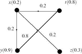
Degree of a vertex x in GDFG1 is the pair (d+(x),d−(x)) where d+(x), out degree of x, is the sum of the generalized membership values of outgoing edges and d−, in degree of x, is the sum of the generalized membership values of incoming edges. Thus,
Note 2 In GDFG1, out degree or in degree of a vertex may be 0. But, when both are 0 then the vertex is called null vertex.
Generalized directed fuzzy graph of second kind (GDFG2) is introduced below.
Definition 4.
Let V be a non-empty set. Two functions are considered as follows. ρ : V → [0,1] and Let
From the definition it is clear that, if a vertex has no incoming edge but has outgoing edges, its generalized membership value is 0. Let us discuss this situation with an example.
Example 2.
Here, V = {a,b,c,d,e}.The edge membership values are given as
A generalized directed fuzzy graph of second kind (GDFG2)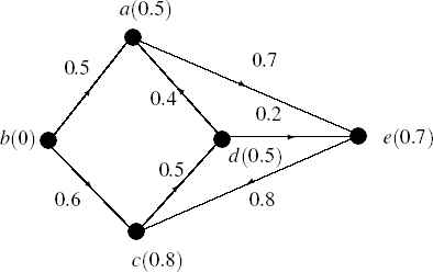
Degree of a vertex x in GDFG2 (similarly defined) is the pair (d+(x),d−(x)) where d+(x), out degree of x, is the sum of the generalized membership values of outgoing edges and d−, in degree of x, is the sum of the generalized membership values of incoming edges. Thus,
Note 3 In GDFG2, in-degree or out-degree of a vertex may be zero. If both of them are zero, the vertex is said to null vertex.
3.2. Isomorphism in GFGs
The definition of homomorphism is given first.
Definition 5.
Let ξ1 = (V1,ρ1,ω1) and ξ2 = (V2,ρ2,ω2) be two GFG1 (or GFG2). Also let, h : V1 → V2, θ1 : A1 → [0,1] and θ2 : A1 → [0,1] be the functions where A1 = {ρ2(x)|x ∈ V2} and A2 = {(ρ2(x), ρ2(y))|x,y ∈ V2, (x,y) is an edge in ξ2} such that ρ1(x) = θ1(ρ2(h(x))) and ω1(x,y) = θ2(ω2(h(x),h(y))). Then, the function h is said to be homomorphism between two generalized fuzzy grtaphs.
If two systems are equal in vertex and edge membership values, then they are called isomorphic.
Definition 6.
Let ξ1 = (V1,ρ1,ω1) and ξ2 = (V2,ρ2,ω2) be two homomorphic GFG1s (or GFG2s). Also let, h : V1 → V2, be a bijective homomorphism and θ1 and θ2 are both identity mappings. Then, the function h is said to be isomorphism between two generalized fuzzy graphs.
Example 3.
Let us consider a GFG1, ξ1 =(V2,ρ1,ω1) where V1 = {a(0.6), b(0.5), c(0.7), d(0.8)} and edge set {((a,b),0.5), ((b,c),0.5), ((c,d),0.7), ((d,a),0.8)} which is shown in Fig. 3(a). Also, let another GFG1, ξ2 = (V2,ρ2,ω2) V2 = {a′ (0.6), b′ (0.5), c′ (0.7), d′ (0.8)} and edge set {((a′,b′),0.5), ((b′,c′),0.5), ((c′, d′),0.7), ((d′,a′),0.8)}. Also, let h : V1 → V2 such that h(a) = a′, h(b) = b′, h(c) = c′, h(d) = d′. θ1(x) = x and θ2(y) = y. Then, by routine calculation, it is observed that the graphs are weak isomorphic.
Isomorphism between two generalized fuzzy graphs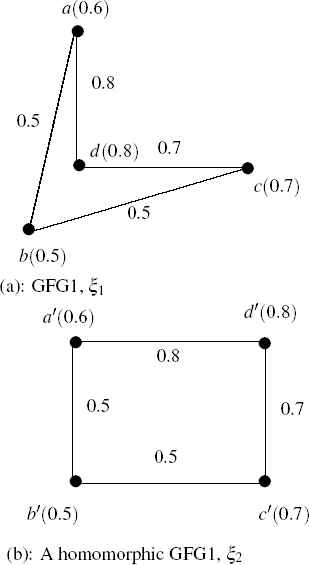
4. Generalized fuzzy competition graphs
Neighbourhood of vertices is a related term to define GFCG.
4.1. Neighbourhood of a vertex in GFG
In GFG, neighbourhood of a vertex is the set of adjacent vertices. Let x be a vertex of a GFG, ξ and x is adjacent to the vertices y1,y2,...,yk. Then, the neighbourhood of x is the set {(y1,ω(x,y1)), (y2,ω(x,y2)),..., (yk,ω(x,yk))}. A vertex y is said to be strong neighbour of x if ω (x,y) > 0.5. In GFDG,
In Fig. 1, neighbourhood of x is {(y,0.9),(z,0.5),(t,0.8)}. In the same figure, the out-neighbourhood of x is the set {(y,0.2),(z,0.2)} and in-neighbourhood of x is (t,0.2).
The neighbours may be indirect also. Suppose, there is a directed path from x to xm of length m as x → x1 → x2 → ... → xm−1 → xm. Then, xm is said to be m-step out neighbourhood of x. Let
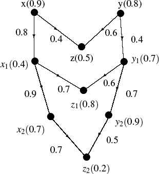
Indirect neighbourhoods
4.2. Generalized fuzzy competition graphs
Definition 7.
Let ξ = (V,ρ,ω) be a GFDG. Now, the generalized competition graph of ξ is a GFG, C(ξ) = (V,ρ′,ω′) where ρ′ = ρ. Also,
Example 4.
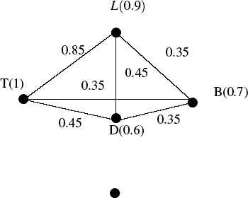
Let us consider a competition among Tiger(T), Lion(L), Dog(D), Bear(B) for Food(F) (see Fig. 5). Here, the predators and prey are assumed as vertices, i.e. V = {T,L,D,B,F}. The membership values of the vertices are taken as their strengths for snatching the food. Suppose ρ(T) = 1, ρ(L) = 0.9, ρ(D) = 0.6, ρ(B) = 0.7, ρ(F) = 0.35. Also, the demands of the particular food for the predators are taken as edge membership values. Empirically,
Competition among predators. GFCG of Fig. 5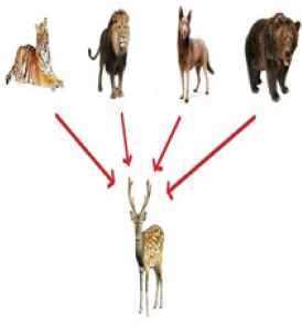
GFCG represents any competition with much effective way. Any GFG may be considered as GFCG of some GFDG. This GFDG may not be unique. The following theorems clarify the statement.
Theorem 1.
Let ξ be a GFG. There exists a GFDG,
Proof.
Let ξ = (V,ρ,ω) be a GFG and (x,y) be an edge of the graph. Now, a GFDG,
There may be more than one GFDGs which satisfies Theorem 1. An example is given below. In Fig. 7(a), a GFG is shown. In Fig. 7(b) and Fig. 7(c), GFDGs are shown whose GFCG is the same graph of Fig. 7(a). By routine calculation, this is easy to understand. So there are infinitely many GFDGs whose competition graph is ξ.
GFDGs in (b), (c) and their GFCG in (a)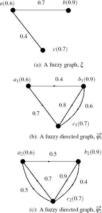
Among the GFDGs whose competition graph is a given GFG, some types of graphs have minimum number of edges. These graphs are called minimal graphs which are defined below.
Definition 8.
Let ξ be a GFG. Minimal graph,
Example 5.
In Fig. 7(b), the number of edges of the graph,
Minimal graphs of any GFG are not unique. Infinitely many GFDGs can be constructed with different edge membership values. But all the minimal graphs have same number of edges. The underline crisp graphs of the minimal graphs of a GFG are isomorphic. Thus, there exists one-one map-pings between vertices and edges between the minimal graphs.
Theorem 2.
Let (x,y) be an edge in a GFG, ξ = (V,ρ,ω). Also, let
Proof.
Let (x,y) be an edge in a GFG, ξ = (V,ρ,ω) and
Theorem 3.
Isomorphic GFDGs are minimal graphs of some GFGs, but minimal graphs are not necessarily isomorphic.
Proof.
The isomorphic graphs have equal number of edges. The membership values of corresponding vertices and edges of the isomorphic graphs are equal. Thus, if one GFDG is minimal graph of some GFGs, then all other isomorphic graphs are minimal. But, the converse may not be true. If (x,y) is an edge in a GFG, ξ = (V,ρ,ω) and
The characterization of minimal graphs such as the number of possible edges are discussed below.
Theorem 4.
Let ξ be a given connected GFG whose underlying graph is a cycle with m edges. The number of edges in minimal graphs of ξ is equal to 2m where m ⩾ 3.
Proof.
Let ξ be a given connected GFG whose underlying graph is a cycle with m edges. Let x1,x2,...,xm be the vertices of ξ. Also, let y1,y2,...,ym be the corresponding vertices in a minimal graph
A GFG with m edges and its minimal graph with 2m edges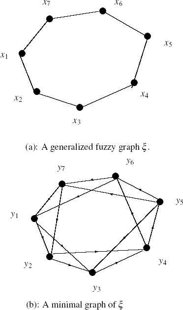
Theorem 5.
Let ξ be a given connected GFG whose underlying graph is a complete graph with n vertices. The number of edges in minimal graphs of ξ is equal to 2n where n ⩾ 3.
Proof.
Let ξ be a given connected GFG whose underlying graph is a complete graph of n vertices. Every vertices of ξ are connected with each others. Let x,y be two adjacent vertices in ξ and x1 and y1 be the corresponding vertices in the minimal graph
A GFG (whose underling graph is complete) with n vertices and its minimal graph with 2n edges.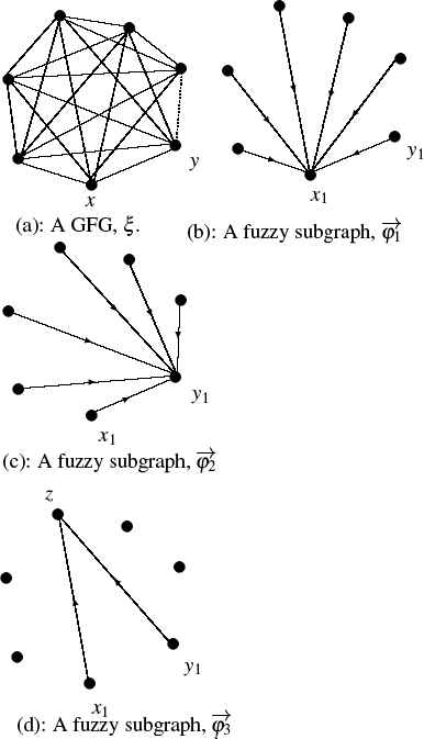
It is an important task to calculate the number of edges in a minimal graph of a given graph. It is easy to prove that the number of edges of a minimal graph is less than or equal to 2m if the given graph has m edges.
Note 4 Let ξ be a given connected GFG with m edges. The number of edges in minimal graphs of ξ is less than or equal to 2m where m ⩾ 4.
Let ξ be a connected GFG with m edges where m ⩾ 4. If underline graph of ξ is a cycle, then the number of edges in minimal graph is twice the number of edge in ξ. Again, underline graph of ξ is complete graph, then number of edge is twice the number of vertices. For n ⩾ 4, the number of edges of such GFG is greater than its number of vertices. This concludes the result.
Note 5 Let ξ be a given connected GFG with m edges where m ⩽ 3. The number of edges in minimal graphs of x is equal to 2m.
5. Real life problem by GFCG
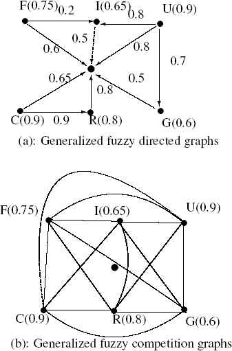
Competition is arising in every aspect of life. Here an example of real life competition among the countries for economic growth is given. The countries {France(F), India(I), USA(U), Russia(R), China(C), Germany(G)} are considered here. In Fig. 10, the competition is shown. The graphical representation of the competition is shown in Fig. 11 (a). Now, the competition among the countries is shown in Fig. 11 (b). Suppose the competition between U and C is to be calculated. In Fig. 11 (a), U has direct edge to E(economy) with membership value 0.8 and has indirect edge (2-step) 0.8 × 0.5 = 0.4. So out neighbourhood of U is E with membership value 0.8. Now, C has direct edge to E with membership value 0.65 and indirect edge with membership value 0.9 × 0.8 = 0.72. Thus out neighbourhood of C is E with membership value 0.72. As indirect out neighbourhood of C is strong, so its membership is considered. Hence, there is a competition between U and C. The membership value of the edge between U and C in corresponding competition graph is 0.72 according to the Definition 7. And all other edges in corresponding competition graph is shown in Fig. 11 (b).
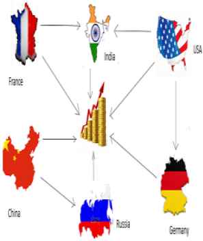
Competition for economy among some countries
Generalized fuzzy competition graphs
6. Insights for this study
- •
Edge restrictions on fuzzy graphs are removed
- •
The relations between vertex and edge membership values are established.
- •
The concept of neighbourhood is modified and more generalized.
- •
Competition graphs are generalized.
- •
Minimal graphs are introduced. Some competitions are almost same. These competitions are represented by minimal graphs.
- •
An example is shown in Example 4 to show prey-predators competition in forest.
- •
Some theorems are proved regarding minimal graphs. These theorems are helpful to build algorithms to find the number of vertex and edges in a minimal graphs of any large competitions.
- •
An example is shown in Section 5 to show the competition on economy among different countries.
7. Conclusions
This study described some major properties of generalized fuzzy directed graphs. The concepts of neighbourhood of vertices were generalized for those graphs. Indirect neighbourhood may get preference over direct neighbourhood if the product of membership values of edges in indirect path is greater than membership value of direct edge. After that, concept of competition graphs was generalized. This study also introduced another important graph namely minimal graphs and their properties. The concept of minimal graph depended on number of edges. But, the concept can be extended depending on membership values of edges also. These representations are helpful to understand the real life competitions. In near future, the important properties and related algorithms will be established. Also, multi-label competitions must be represented by some graphs. This paper will be backbone for that.
References
Cite this article
TY  - JOUR
AU  - Sovan Samanta
AU  - Biswajit Sarkar
PY  - 2018
DA  - 2018/03/02
TI  - Representation of competitions by generalized fuzzy graphs
JO  - International Journal of Computational Intelligence Systems
SP  - 1005
EP  - 1015
VL  - 11
IS  - 1
SN  - 1875-6883
UR  - https://doi.org/10.2991/ijcis.11.1.76
DO  - 10.2991/ijcis.11.1.76
ID  - Samanta2018
ER  -