
Dynamic deep learning algorithm based on incremental compensation for fault diagnosis model
- DOI
- 10.2991/ijcis.11.1.64How to use a DOI?
- Keywords
- Deep learning; Dynamic compensation; Fault diagnosis; Denoising Autoencoder; Incremental learning
- Abstract
As one of research and practice hotspots in the field of intelligent manufacturing, the machine learning approach is applied to diagnose and predict equipment fault for running state data. Despite deep learning approach overcomes the problem that the traditional machine learning approaches for fault diagnosis is difficult to characterize the complex mapping between the massive fault data, the exponentially grown and newly generated data is learned repeatedly, and these approaches cannot incrementally correct the model to adapt the situation that the states and properties of equipment are changed over time, resulting in the increase of time costs and the decrease of diagnosis accuracy of model. In this paper, a dynamic deep learning algorithm based on incremental compensation is proposed. Firstly, the feature modes of the newly generated data are extracted by using deep learning algorithm; it is then compared with the fault modes extracted from the historical data. Next, a similarity computing model is presented to dynamically adjust the weights of incrementally merged modes. Finally, the SVM algorithm is employed to classify the weighted modes by supervised way, and the BP algorithm utilized to fine tune the model, in order to complete the dynamic and compensatory adjustment of deep learning with original modes and incremental modes. The experimental results of bearing running data demonstrate that the proposed approach could significantly improve the accuracy of diagnosis and save the time cost, contributing to meet the varied needs of the real-time equipment fault diagnosis.
- Copyright
- © 2018, the Authors. Published by Atlantis Press.
- Open Access
- This is an open access article under the CC BY-NC license (http://creativecommons.org/licences/by-nc/4.0/).
1. Introduction
Under the background of the Industry 4.0, it is gradually crucial to figure out how to extract the feature information of fault from the equipment running state data and make an effective analysis to achieve the fault diagnosis and prediction, which has become a hotspot in the field of intelligent manufacturing. At the same time, with the development of the industrial Internet of things and information technology, massive running state data emerge in the process of production, making it possible to use big data analysis approach for fault diagnosis.
In recent years, with the increase of the equipment running state data, more and more worldwide researchers have applied machine learning approaches to the field of equipment fault diagnosis. Most of the traditional machine learning approaches are shallow learning, such as neural network1, 2, support vector machine3, 4 and clustering5. These approaches can efficiently solve the problem that the mapping structure is relatively simple or the small sample is given multiple constraints; while faced with the complex problems from massive data, it will be difficult for them to extract the abstractly implicit features between multiple fault modes, and the convergence rate will be slow and easy to fall into the local optimum. Therefore, the traditional machine learning approaches has the limitations and is not suitable for handling the booming equipment state data. More recently, deep learning has made great achievements in the field of image processing and speech recognition with its strong modeling and characterized capabilities6–8. At present, some scholars have investigated deep learning to equipment fault diagnosis9–12, which effectively addresses the problems of traditional fault computing model. With the rapid development of industrial Internet of things, the deep learning approaches have new problems: Because of the exponential growth in the size of newly generated equipment state data, it is clearly unreasonable to rely on existing fault modes for matching. Therefore, how to mine the newly generated state data and merge it into the mining model of the existing de ep learning algorithm becomes a new problem. The approach of merging all data to re-train model and mine again is very time-consuming, which is not suitable for equipment fault diagnosis and prediction with strong real-time performance. Thus, incremental learning becomes the first choice to solve this problem and it has many approaches and models, such as incremental extreme learning machine (IELM)13, 14, online incremental learning support vector machine (OISVM)15, online learning neural network model (ONN)16, etc., it has achieved better effect of incremental mining in the existing literatures. However, in the field of fault diagnosis, the state and properties of the equipment will change over time, thus the newly generated data which at the recent time point has more important value for mining fault modes; meanwhile, some determined fault modes may also become invalid along with machine state changes. These characteristics hinder the further application of above incremental approaches in the field of equipment fault diagnosis.
Through the above analysis, we consider to conduct a fault diagnosis model with dynamic deep learning algorithm based on incremental compensation (ICDDL). Firstly, denoising autoencoder (DAE) algorithm of deep learning is developed to extract feature modes from newly generated data. Then, for comparing the new modes with the modes extracted from the historical data, the proposed approach further provides a computation of similarity measure based on Kullback - Leibler divergence (KL Divergence), and adjusts the weights of modes dynamically according to the different similarities. Finally, the weighted modes are classified by supervised SVM algorithm, and the parameters of whole networks are fine-tuned by BP algorithm according to the error of model. Compared with the traditional deep learning algorithms, the proposed approach not only emphasizes the new fault modes, but also takes the original invalid modes into account, so as to achieve the dynamic and compensatory adjustment of deep learning with original modes and incremental modes.
The proposed ICDDL approach utilizes feature weighting to measure the varying degree of the significance of feature modes with the time and state changed between original modes and incremental modes, and it achieves fault diagnosis of bearing running data. The innovation of proposed approach is illustrated in the following. First, a dynamic deep learning approach is proposed to dynamically adjust the weights of the feature according to the difference between the new feature modes and the existing feature modes, and effectively complete the incremental learning of the newly generated state data. Second, a computing model of similarity measure based on KL divergence is introduced to compute the similarity degree of feature, and further iterate the weight value of feature. Third, the study implements the dynamic learning and incremental learning of equipment fault modes, which could extract feature and diagnose fault for the newly generated data from the real-time operation of equipment, and solves the problem that the new state of equipment caused by abrasion is not considered by original fault modes, improving the reliability of diagnosis model.
The remainder of this paper is organized as follows: Section 2 summarizes the related literature of the research on fault diagnosis approaches, deep learning and incremental learning. Section 3 illustrates the theoretical basis, flow, and the step of implementation of the proposed dynamic deep learning algorithm based on incremental compensation (ICDDL) model in detail. Section 4 applies the ICDDL approach to the process of fault diagnosis for bearing equipment, and achieves the real-time extraction of state feature and the reliable classification of fault modes for bearing equipment. The validity of the ICDDL approach is proved by experiment. Finally, the brief summary of proposed approach and the potential future research directions are described in Section 5.
2. Literature Review
The current researches of equipment fault diagnosis, deep learning and incremental learning are summarized as follows.
2.1. Equipment fault diagnosis
At present, intelligent equipment is widely used in industry, aviation, national defense and other vital areas, and the consequences of fault are relatively serious, thus how to carry out reliable fault diagnosis and prediction has attracted extensive attention. Especially with the advent of the era of industrial Internet of things, the approach based on data analysis has become the mainstream of that field, and many scholars have a deep research on it1–5, 17, 18. H. Fernando et al.2 proposed an unsupervised artificial neural network for fault detection and identification based on Adaptive Resonance Theory (ART). The performance and practical ability of approach for detecting and identifying known, unknown and multiple faults are superior to the traditional rule-based approaches. Y.S. Wang et al.4 developed a HHT–SVM model for intelligent fault diagnosis of engine noise feature. The Hilbert–Huang transform was exploited to the measured noise signals as the input vector to construct an optimal SVM model. It could deal with both the stationary and nonstationary signals and even the transient ones very well. The aforementioned machine learning algorithms utilize complex mapping function modeling and parameter space searching optimization to improve the accuracy of equipment fault diagnosis effectively; nevertheless there are some problems in uncertain relation of map and difficult selection of parameter. The fuzzy evaluation could give a quantitative evaluation of non-deterministic fuzzy problems. Combining it with the machine learning algorithm can improve the performance of models, enhance the adaptability of models and solve the uncertain problems. S. Yin et al.5 utilized principal component analysis to confirm the number of clusters of fuzzy positivistic C-means clustering for detecting faults of vehicle suspension, and then demonstrated the effectiveness of the approach. Another way to improve the performance of machine learning is the Hidden Markov model, which can find the hidden parameters of model through probabilistic reasoning. M. Yuwono et al.18 proposed an automatic bearing defect diagnosis approach based on Swarm Rapid Centroid Estimation (SRCE) and Hidden Markov Model (HMM). It achieved an increase in average sensitivity and specificity and a reduction in error rates.
It can be seen from the above literature that the data analysis approaches have achieved good results in the field of equipment failure; however, in recent years, with the increase of the scale of monitoring group, measuring points and sampling frequency, the equipment condition monitoring data grew substantially. Although the traditional shallow models could efficiently solve the problem that the mapping structure is relatively simple or the small sample is given multiple constraints, they still could not meet the requirements when deal with the complex problems caused by the data streams of massive, heterogeneous and multi-source. Hence, deep learning has been paid more attention to in order to represent the complex functions of high order and abstract concepts and solve the task related massive data.
2.2. Study on deep learning in fault diagnosis
The concept of deep learning is highly valued by academics with its powerful abilities of modeling and characterizing since it was put forward. As deep learning extracts the different levels feature of the original data from the hierarchical processing of input data, it facilitates the multi-level simulation of step-by-step computation for the fault prediction. Meanwhile, the multi-level extracted features obtained by the deep learning could be repeatedly used in similar different tasks, which are conducive to get more useful information for equipment fault diagnosis. At present, some scholars have investigated deep learning theory to the field of equipment fault diagnosis, P. Tamilselvan et al.9 presented a novel multi-sensor health diagnosis approach using deep belief network (DBN). The DBN employed a hierarchical structure with multiple stacked Restricted Boltzmann machines and worked through a layer by layer successive learning process to diagnosis the healthy state of equipment. The experimental results showed that the approach had better accuracy than that of the shallow machine learning approaches. However, thisapproach still extracted the fault feature manually, and only used the deep belief network as a classifier, ignoring its ability of mining fault features. On the basis of those approaches, F. Jia et al.10 constructed a deep neural network (DNN) by stacking five level autoencoders and used it to extract fault feature and diagnosis fault intelligently for rotating machinery spectrum. The approach was validated using datasets from rolling element bearings and planetary gearboxes that it had higher diagnostic precision compared with the existing shallow model. But they only apply the existing deep learning approach to equipment and did not adapt to the particularity of equipment state data. While M. Gan et al.11 proposed a construction of hierarchical diagnosis network based on deep learning. The two-layer deep belief network was utilized to identify the fault location and rank the fault severity of the rolling bearing, respectively. However, there was a problem that the second layer results of fault severity ranking depended on the accuracy of the first layer fault location recognition. The deep random forest fusion (DRFF) model proposed by C. Li et al.12 happened to be able to make up for the shortage of the above problems. Two deep Boltzmann machines (DBMs) were developed for the acoustic signal and vibratory signal of gearbox to extract the deep feature, respectively. A random forest was finally suggested to fuse the outputs of the two DBMs to get diagnostic results. The addressed approach improves the fault diagnosis capabilities for gearboxes.
In summary, the deep learning has a stronger ability of representation than the shallow model, and it is more suitable for processing the equipment state data with complex structure and tremendous amount. With the development of the industrial Internet of things, the number of newly generated state data for equipment is proliferated, and even more than the amount of historical data. When processing the newly generated data, the existing deep learning approaches need to combine it with the original data to re-train the whole model, which undoubtedly increases computational complexity and consumes unnecessary time. Therefore, how to mine the newly generated state data and make it combine with the original fault modes has become an urgent problem to be solved.
2.3. Study on incremental learning in fault diagnosis
The problem of processing the new state data could be attributed to an incremental learning problem. Incremental learning means that a learning system could continuously learn new knowledge from new samples and could also keep most of the knowledge that has been learned previously. Incremental learning, as a very active research field, has been derived from a variety of incremental mining approaches to reduce the computation, improve the accuracy of models, and save time cost effectively. G. Yin et al.19 proposed an online fault diagnosis approach based on Incremental Support Vector Data Description (ISVDD) and Extreme Learning Machine with incremental output structure (IOELM). Nevertheless, in this model a priori knowledge should be provided to help make decision in the determining process. Taking into account the prior knowledge is difficult to obtain, H.H. Chen et al.20 utilized the model space learning and the incremental one class SVM to diagnose fault of the TE process. It constructed the fault dictionary in real time by sliding windows, and put the new data which is not in the existing model into the candidate pool. This approach built a new one class until the number of data point in the candidate pool exceeded half the size of the sliding window. However, the fault which the model found was more than the actual existence due to the lack of fault information. Therefore, aimed at the problems that the data tend to be online imbalanced, W.T. Mao et al.13 proposed an online sequential prediction approach for imbalanced fault diagnosis problem based on extreme learning machine. This approach introduced the principal curve and granulation division to simulate the flow distribution and overall distribution characteristics of fault data, respectively. Then in online stage, the obtained granules and principal curves were rebuilt on the bearing data which arrived in sequence, and after the over-sampling and under-sampling process, the balanced sample set was formed to update the diagnosis model dynamically. On its basis, J. Liu et al.21 introduced an adaptive online learning approach for support vector regression (Online-SVR-FID). The approach adaptively modified the model only when different pattern drifts were detected according to the proposed criteria. Additionally, it judged the current mode could be represented by a linear combination of the existing modes or not to determine to change the existing modes or add new modes.
In summary, the different incremental learning approaches all have further improved the efficiency of mining modes. With the continuous improvement of industrial automation, the number of equipment state data is proliferated, and the newly generated data has a more important value for estimating the trend of fault. Up to now, deep learning approaches have already had a better performance in the field of equipment fault diagnosis, and it is more important to study the incremental mining of deep learning to further improve the accuracy of model. Therefore, a dynamic deep learning algorithm based on incremental compensation is proposed in this paper. Compared with the traditional mining mode of increment learning, this proposed approach is not only beneficial to strengthen the effective fault modes in the original fault sets, but also conducive to reduce the fault modes which get invalid with the change of equipment state. The proposed approach meets the specific requirements of equipment fault diagnosis, so it has great research value.
3. Dynamic Deep Learning Algorithm Based on Incremental Compensation
In this section, the ICDDL approach is introduced in detail. The approach firstly extracts the feature mode from the newly generated data by using the denoising autoencoder22, and it further proposes a similarity computing approach, which compares the new modes with the existing modes; next it adjusts the weights of modes dynamically according to the different similarities. Finally, the weighted modes are classified by supervised SVM algorithm, and the parameters of entire networks are fine-tuned by BP algorithm according to the error of model.
3.1. Dynamic compensation of incremental learning
As the primary step of ICDDL approach, the dynamic compensation of incremental learning is mainly composed of three steps: similarity computation of modes, increment and merged of modes and computation of dynamically compensatory weight. It could effectively solve the problem of the change of the feature modes caused by the variance of the state data and property with the abrasion of equipment.
3.1.1. Similarity computation of modes
Aiming at the particularity of high dimension and complexity of equipment fault modes, this paper proposed a similarity computing approach based on KL divergence. The approach could effectively distinguish objects that are difficult to be distinguished by geometric distance, and could improve the applicability and accuracy of similarity for fault modes.
KL divergence23, also known as the relative entropy, is used to measure the difference between distribution P and Q. For discrete distributions, the KL divergence of P and Q is defined as Dkl(P‖Q)
It can be seen that the smaller KL divergence between P and Q is, the greater value of the above equation will be, that is, the higher similarity between the features will be, so as to measure the similarity of the newly generated feature modes and original feature modes.
It is known from the nature of KL divergence that it has no symmetry, that is Dkl(P‖Q) ≠ Dkl(Q‖P), but it needs symmetry when it is represented the similarity between two features. To this end, the symmetry of KL divergence is modified by
In the computation of KL similarity between the features, Dkl(P‖Q) in Eq. (2) is replaced by Dkls (P‖Q) as
As the KL divergence is computed the dissimilarity based on the relative entropy between distributions, rather than through the distance measure, it can effectively distinguish objects that are difficult to be distinguished by geometric distance. Being superior to other distance-based similarity measures, it could accurately measure the degree of similarity between fault modes.
3.1.2. Increment and merged principles of modes
The KL similarity between the new feature modes and the original feature modes is computed by using Eq. (4), and the maximum value of Sim(P, Q)max is served as the mode similarity value of feature. In general, the determination of generating or merging the mode is according to the following principles:
α is a symbol for the minimum similarity threshold which makes the similarity between two contrast features meaningful, and its value is α = minSim(Fi, Fj), which represents the minimum similarity between two features Fi and Fj in the existing feature modes. β is used to stand for the critical threshold between general similarity and high similarity of feature, and its value is β = maxSim(Fi, Fj), which represents the maximum similarity between two features Fi and Fj in the existing feature modes. It can be seen that with the similarity threshold α < β, the threshold α and β are dynamically changed with the increment and merge of feature modes.
- (i)
If β < Sim(P, Q)max, it means that the new features are highly similar to those in the original modes, and these features should be merged by harmonic non-linear weighted averaging approach;
- (ii)
If α < Sim(P, Q)max < β, it means that the new features are different from all the existing ones. And the new feature should not be replaced by merging with the existing features. So this feature is incrementally generated to the existing modes;
- (iii)
If Sim(P, Q)max < α, it means that the similarity between the new feature and the existing feature is lower than the minimum threshold, which reveals the new feature is meaningless noise or disturbance value to be abandon.
3.1.3. Computation of dynamically compensatory weight
According to the principles of increment and merged for new modes, the dynamic compensation of weights are computed to measure the degree of importance changed over time for feature modes, and to enhance the effective modes and reduce the invalid modes in the form of weight compensation. Since the similarity of the new feature and the existing feature can reflect the importance of the new modes to the current model in a certain extent, the similarity value of modes is normalized using Eq. (5) and is computed for dynamic weight.
The principle of (i) for high similarity modes are took the merge operation. It shows that these modes are frequently appeared with the process of varying equipment state, and these modes are so essential that should increase their weights to enhance the effective modes. The dynamic weight computing approach is as follows, where the greater similarity of feature, the more important function of the feature in the modes.
The principle of (ii) for features which have incrementally added to the original modes are took newly generate operation. It shows that these modes are newly generated with the change of state data and need to be given the initial weights computed by following approach, where the importance of feature in current model happens to be able to represent by the similarity of feature.
The principle of (iii) for new modes which are abandoned are not took into account, but there are cases where the similarity of original modes with all the new features is less than the threshold α, which indicates that it does not appear in the new modes, and these original modes are gradually became invalid with the variance of state data. Therefore, the weights are slowly reduced by using Eq. (8). After several iterations of incremental learning, the weights of the feature that have not appeared will gradually decrease until it is less than the threshold α, indicating that the feature has become invalid and it needs to be removed from the existing modes.
Through the above computation scheme of weights, feature weights are dynamically adjusted in each comparison between the original modes and the new ones. The variance degree of importance for feature modes with the change of state data are compensated by using similarity, to achieve the goal ultimately that the effective modes are preserved and enhanced and the invalid modes are removed and decreased.
3.1.4. Increment learning based on dynamic compensation
Because of the incremental learning approach need not to preserve the historical data, the storage space has saved. Meanwhile, the time cost for modifying a trained system is generally much lower than the cost of retraining a system, so the computing resources are saved. Therefore, this paper proposes an incremental learning approach based on dynamic compensation.
The incremental learning process based on dynamic compensation is shown in Fig. 1. Firstly, the new feature modes are mined and extracted from the newly generated data by using the trained DAE model. Secondly, the similarity value of the new modes and original modes is computed by the similarity computing approach in Section 3.1.1, and the increment or merge operation of the new mode is determined depends on the similarity. Then, the dynamically compensatory weights are computed by using the scheme in Section 3.1.3. Finally, the new modes are input into the classifier together with the original feature modes, and the parameters of model are adjusted to complete the process of incremental learning. Compared with the traditional incremental mining, the dynamic compensation of incremental learning approach assigns the dynamic weights to the equipment state data at different time points. The effective modes are improved and the invalid modes are reduced in the form of weight compensation.
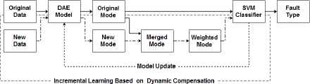
Incremental learning process based on dynamic compensation
3.2. Dynamic deep learning based on incremental compensation
Deep learning approaches generally layer-by-layer pre-train the deep network structure to extract the features with unsupervised learning approach at first. A classifier is then added to the top layer of the deep network to classify the feature modes. Meanwhile, the parameters of model are fine-tuned to further optimize the training results by back propagation algorithm with supervised learning. Considering the complex environment of equipment, the noise and information redundancy of state data, the denoising autoencoder22 which could remove the noise and disturbance is served as the unsupervised algorithm in the pre-training procedure. The Support Vector Machine (SVM) is selected as the classifier because of its excellent performance of classification for high-dimensional and complex data.
3.2.1. Denoising autoencoder
Because of the complexity of the environment, most of equipment state data contain noise and information redundancy, it is very essential to figure out how to force the hidden nodes to find more robust features and effectively avoid learning identity function to improve the accuracy of fault diagnosis. DAE based on the Autoencoder24 (AE), is trained by adding noise which contains certain statistical features to the input samples, and the original form of disturbed samples is estimated through output layer, so as to obtain more robust feature from the samples contained noise.
The autoencoder, a kind of three-layer neural network, includes input layer, hidden layer and output layer. It is composed of encoding network and decoding network as shown in Fig. 2. The output target and input data of AE are as same as possible. The input data from high-dimensional space is transformed into coding vectors in low-dimensional through the hidden layer, and then the coding vectors are reconstructed to original inputs. The object is to make the reconstruction error minimum, and then the code vector could be regarded as feature representation of input data.
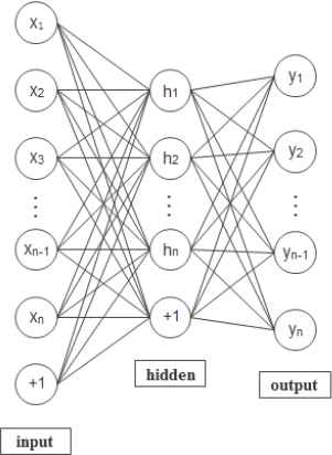
Structure of AE
Given an unlabeled n-dimensional sample set x as the input of autoencoder model, the mapping relationship from input sample to hidden layer is denoted by h, and the mapping relationship from hidden layer to output layer is denoted by y. Thus the mapping function between the input layer and the hidden layer could be defined as
The reconstruction error function L(x, y) in the above equation is adopted the cross entropy loss function as following
The procedure of denoising autoencoder is shown in Fig. 3. Firstly, the random noise is added to sample x according to the distribution of qD, which makes it become the noisy sample
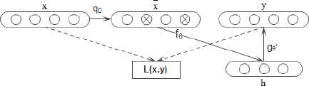
Procedure of denoising autoencoder
3.2.2. Dynamic deep learning based on incremental compensation
In this paper, the deep learning approach is performed to construct a deep network structure by stacking multi-layer connected denoising automencoders as shown in Fig. 4. The outputs of the lower layer of DAE are treated as the inputs of the next higher layer of DAE, and the coefficients of each layer are greedy trained layer by layer to minimize the cost function. An output layer with classification function is added to the top layer of deep network structure, and the SVM is served as the classifier to supervised classification. The fine-tuning procedure enables the deep network to modify the parameters of each layer by BP algorithm through the error, and further optimize the whole network to achieve the global optimum.
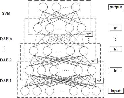
Structure of deep learning network
3.2.3. Flow of algorithm
The steps of proposed dynamic deep learning algorithm based on incremental compensation are described as follows and the flow chart of the algorithm is shown in Fig. 5.
- •
Step 1: The data samples are proportionally divided into training samples and testing samples by random sampling, and the testing samples are labeled. The training samples are divided into four groups. One group is used to train the deep learning model, and the remaining three groups are added to the existing model separately for three times to execute incremental learning based on dynamic compensation;
- •
Step 2: With the parameters of model being initialized, the training samples for training deep learning model are added random noise as the input of denoising autoencoder, to greedy unsupervised pre-train the model layer-by-layer. The feature modes are then extracted from the data samples. The unified and initial weights W0 are given to the feature;
- •
Step 3: If there are no newly generated data samples added, then to Step 4. If there are newly generated data samples added, then the features are extracted from new data by using the existing model to obtain the newly generated feature modes at first. The KL similarity of each feature in the new feature modes and the original feature modes is computed by using the Eq. (4), and the new feature modes are incrementally merged and dynamically weighted according to the following principles in terms of KL similarity:
- (a)
If the KL similarity of newly generated feature is greater than threshold β, it indicates that the feature is highly similar to the existing features, then to develop the harmonic non-linear weighted averaging algorithm to merge them, increasing the weight of feature according to Eq. (6);
- (b)
If the KL similarity of newly generated feature is greater than threshold α, and less than threshold β, it indicates that the feature is a newly generated feature which occurs with time. The feather is then added to the feature set incrementally, and its weight is set according to Eq. (7);
- (c)
If the KL similarity of newly generated feature is less than threshold α, it indicates that the feature has little effect on the existing modes, and it may be a meaningless noise or disturbance value. It will be abandoned;
- (d)
If the KL similarities between original feature and all newly generated features are less than the threshold α, it indicates that the original feature becomes invalid with time. The weight of feature is reduced according to Eq. (8) until it is less than the threshold α, and it will be removed from the current modes;
- (a)
- •
Step 4: The labeled data and the unlabeled data trained and weighted by dynamic deep learning are served as the input vector to train SVM classifier;
- •
Step 5: The relevant parameters of the entire model are globally fine-tuned by using the BP algorithm to achieve the optimal parameters which minimize the value of loss function both in pre-training phase and incremental learning phase of model.
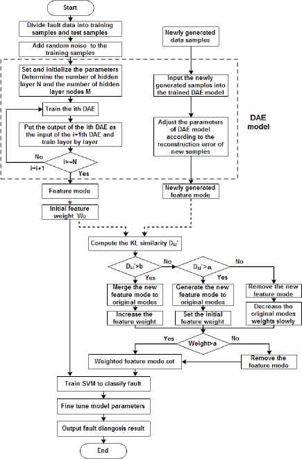
Flow chart of dynamic deep learning algorithm based on incremental compensation
3.3. Application of ICDDL algorithm in bearing fault diagnosis
The specific procedure of dynamic deep learning model based on incremental compensation for bearing equipment fault diagnosis is shown in Fig. 6., and the steps of implementation are as follows:
- •
Step 1: Preprocessing the state data of bearing equipment, and extracting the feature vector for the classification of fault mode after Wavelet Packet Transformation (WPT). The data samples are divided into training samples and testing samples by random sampling, and the testing samples are manually labeled the type of fault. In order to achieve the dynamic compensation of incremental learning, the training samples are equivalently divided into four groups: one group is used to train the deep learning model, and the remaining three groups are added to the existing model separately for three times to execute incremental learning;
- •
Step 2: Initializing the parameters of model, and greedy unsupervised pre -training the denoising autoencoder layer-by-layer with the running data of bearing equipment which added random noise as the input. After extracting the feature modes of fault and giving the unified and initial weights to features, the labeled data and the unlabeled data which have trained and weighted, are as the input vector to train SVM classifier for classified diagnose of bearing fault modes. The relevant parameters of the entire network are fine-tuned by using BP algorithm;
- •
Step 3: When new state data of equipment is generated, the new fault modes will be extracted by the existing model, and the newly generated fault modes will be incrementally merged and dynamically weighted according to the dynamic compensation of incremental learning strategy in Section 3.1. The newly weighted feature modes and the labeled data are then input to the SVM classifier for classified diagnose of bearing fault modes. The relevant parameters of entire network are fine-tuned by BP algorithm according to the model error of incremental learning procedure to complete dynamic deep learning.
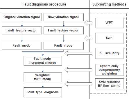
Procedure of fault diagnosis for bearing equipment
4. Experiments
In this section, the application performance of the proposed ICDDL algorithm for bearing fault diagnosis is analyzed by simulation experiments, in order to complete the extraction of state features and the classification of fault modes for bearing equipment. Firstly, the parameters of deep network structure which are suitable for fault diagnosis of bearing equipment are determined by experiments. Then, the validity of ICDDL algorithm is proved by comparing with shallow learning approach as BP, SVM, and deep learning approach without incremental learning as AE and DAE algorithm.
4.1. Data description
The experimental data are bearing fault data which were derived from the Electrical Engineering Laboratory of Case Western Reserve University (CWRU)25. There are 1,341,856 data points in total, and the bearing type is 6205-2RS JEM SKF deep groove ball bearings. A single point fault of three fault levels was set up to the inner ring, the outer ring and the ball of bearing by using Electrical Discharge Machining technology, respectively. The fault diameters were 0.007, 0.014, 0.021 inches. The ten conditions of vibration signals collected by vibration sensor on electric machinery drive end for normal state (N), inner ring fault (IRF), outer ring fault (ORF) and ball fault (BF) are selected and the sampling frequency is 12 kHz. The wavelet packet decomposition is developed to decompose the energy value of each band for the original vibration signals. For each class, 40 samples are selected as training samples and 10 samples as testing samples by random sampling, and each sample contains 2048 data points. The training samples are equally divided into four groups, and one group is used to train the deep learning model, the remaining three groups being added to the existing model separately for three times to execute incremental learning. The specific description of fault data samples is shown in Table 1. The simulation experiment is completed on the computer with Windows 7 64-bit system and Intel-i5 CPU by R3.2.5 platform.
| Class tag | Fault type | Fault diameter (mm) | Training samples | Testing samples | Samples length |
|---|---|---|---|---|---|
| 1 | None | 0 | 40 | 10 | 2048 |
| 2 | IRF | 0.007 | 40 | 10 | 2048 |
| 3 | IRF | 0.014 | 40 | 10 | 2048 |
| 4 | IRF | 0.021 | 40 | 10 | 2048 |
| 5 | ORF | 0.007 | 40 | 10 | 2048 |
| 6 | ORF | 0.014 | 40 | 10 | 2048 |
| 7 | ORF | 0.021 | 40 | 10 | 2048 |
| 8 | BF | 0.007 | 40 | 10 | 2048 |
| 9 | BF | 0.014 | 40 | 10 | 2048 |
| 10 | BF | 0.021 | 40 | 10 | 2048 |
Description of bearing fault data
4.2. Structure of model
The numbers of hidden layers and hidden nodes in deep network structure have great influence on the effect of model. If the number is too small, it may lead to inaccurate extraction of feature and poor results of classification; otherwise, if the number is too large, it will result in exponential increase of computational complexity and much longer running time. Therefore, the number of hidden layers and hidden nodes are determined experimentally in this paper to minimize the reconstruction error of bearing fault diagnosis model.
For the determination of the number of hidden layers, the other parameters of model are set the same and 40 groups of samples for each 10 categories of conditions are selected to experiment on,. The reconstruction error of model is tested by increasing the number of hidden layers from 1 to 10. The experimental results are shown in Table 2., it could be seen that the reconstruction error gradually decreases when the number of hidden layers is gradually increased from one layer, but the reconstruction error increases in fluctuation until the number of hidden layers is increased over four layers. Considering that the computational cost of the model will rapidly increase with the number of hidden layers, this paper selects four layers as the number of hidden layers to construct deep learning network model.
| Hidden layer | Reconstruction error |
|---|---|
| 1 | 0.09205 |
| 2 | 0.06246 |
| 3 | 0.06051 |
| 4 | 0.05865 |
| 5 | 0.05976 |
| 6 | 0.05898 |
| 7 | 0.05849 |
| 8 | 0.05808 |
| 9 | 0.06009 |
| 10 | 0.05831 |
Influence of hidden layer on model reconstruction error
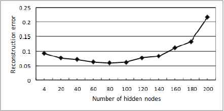
For the determination of the number of hidden nodes, the other parameters of model are set the same, and the number of hidden layers is 4, 40 groups of samples for each 10 categories of conditions are also selected to experiment on. In order to simplify and make the model conform to the characteristics of feature extraction, the numbers of nodes in the 4 hidden layers are set to increase by the ratio of 4: 3: 3: 3 according to the experiment. The variance of model reconstruction error with the increase of nodes number at the first hidden layer is shown in Fig. 7., and the nodes of the rest hidden layers could be estimated by the ratio. It could be seen from Fig. 7., the model reconstruction error decreased with the increase of nodes at the initial stage, but it showed a clearly upward trend when the number of nodes exceeded 80, Therefore, the number of hidden nodes is selected 80, 60, 60, 60, respectively, to construct the deep learning network model.
Influence of hidden nodes on model reconstruction error
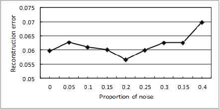
The proportion of noise added to DAE is also one of important factors which affect the effect of model, and the part of useful information may be lost when too much noise are added. Therefore, the parameter value of noise needs to be determined by experiment after constructing the structure of deep network model. The variance curve of model reconstruction error generated with the increase of noise ratio as shown in Fig. 8. It can be seen from the figure, the model reconstruction error has an obviously downward trend when adding 5%–20% of noise. With the gradual increase of the noise, the model reconstruction error increases. It increases so obviously that reaching 0.06985 when the added noise is over 35%. Therefore, the DAE model is constructed by adding 20% noise.
Influence of noise proportion on model reconstruction error
From the above experimental results, the network structure of bearing fault diagnosis model based on ICDDL approach is composed of six layers, including input layer, four hidden layers and output layer. The number of nodes in the input layer is the same as the dimension of feature vector for bearing fault, and the numbers of hidden nodes are 80, 60, 60, 60, respectively. The number of nodes in output layer equals the number of fault categories for bearing. The model is set by adding noise at the proportion of 20%, and the rest of parameters are set to 100 of iterative times and 0.1 of learning rate.
4.3. Experimental results
Based on the model structure defined in above section, all of 400 training samples in 10 different fault states are divided into four groups. The proposed ICDDL approach is used for incremental learning by comparing with BP, SVM, AE, and DAE, respectively. The testing samples are used to test the diagnosed results of the model. The accuracy and running time of each incremental data group are experimented 10 times to compute the average value, and the comparison of average value for four incremental data groups are shown in Table 3.
| Approach | Training accuracy | Training time | Testing accuracy | Testing time |
|---|---|---|---|---|
| ICDDL | 96.85% | 6′20″ | 90.42% | 0.10″ |
| BP | 90.35% | 19′11″ | 67.00% | 1.02″ |
| SVM | 89.18% | 3.97″ | 78.55% | 1.21″ |
| AE | 91.75% | 12′02″ | 85.80% | 0.30″ |
| DAE | 94.41% | 10′21″ | 88.45% | 0.13″ |
Comparison of fault diagnosis results
From Table 3., the proposed ICDDL approach is substantially superior to the other four algorithms in terms of accuracy and running time of model. From the aspect of diagnostic accuracy of model, the ICDDL approach reaches 96.85% in the training phase and 90.42% in the testing phase. Compared with the shallow layer algorithm of BP and SVM, the accuracy of the proposed approach is improved by 6.5% and 7.67%, respectively. It is also improved 2.44%–5.1% by comparing with the deep AE algorithm and the DAE algorithm. With the variance degree of importance for feature modes which changed over time being taken into account, it can be seen that the fault diagnosed accuracy of proposed ICDDL model has a great improvement to a certain extent because the incremental feature modes are weighted by dynamic compensation. From the aspect of running time of model, the proposed ICDDL approach outperforms other algorithms in training time and testing time, except that the training time is longer than SVM algorithm because the time cost for constructing the deep model is contained. The increase of running time is due to that the other four algorithms need to retrain the existing model in the face of incremental data indicating that the dynamic compensation of incremental learning has played a certain role in reducing the computation of model and saving the cost of time. The comparison of proposed DAE algorithm with dynamic compensation of incremental learning and the DAE algorithm without incremental learning for training accuracy and training time is shown in Fig. 9. It could be clearly seen the high efficiency of proposed approach.
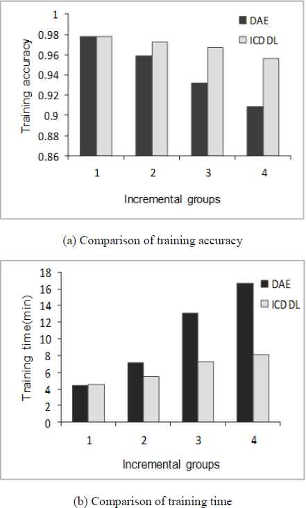
Comparison of model performance for incremental data diagnosis of DAE and ICDDL
Next, the training of incremental data each added is analyzed. The curve of each training accuracy and training time are shown in Fig. 10. that 400 training samples are divided into four groups to be successively added to the model. The proposed ICDDL approach is similarly compared with BP algorithm, SVM algorithm, AE and DAE algorithm without incremental learning. Fig. 10. (a) shows that although the training accuracy of the proposed ICDDL algorithm is not very different from the other four algorithms at the initial stage, the advantage of proposed ICDDL algorithm is more and more obvious with the gradual generation of incremental data by comparing with the other non-incremental learning algorithms. Fig. 10. (b) shows that the proposed ICDDL algorithm requires more time than the SVM algorithm in the initial training, and is basically equal to the AE algorithm and the DAE algorithm, which is due to the training of deep network structure is more complex than shallow models. However, it is obvious that the training time cost by ICDDL algorithm is less than the other algorithms except SVM in the phase of incremental data added. Although the running time required by SVM algorithm for incremental learning is little, the training accuracy are substantial declined with the incremental data added.
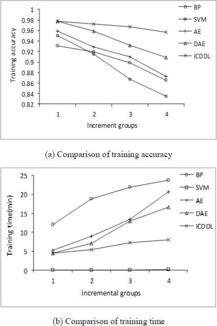
Comparison of model performance for incremental data diagnosis of ICDDL and the other four algorithms
It could be seen that the proposed ICDDL approach has advantages in both accuracy and running time of model compared with the approaches without process of incremental learning. Besides, the proposed fault diagnosis model in this paper could incrementally merge and dynamically weight the newly generated feature modes through dynamic compensation of incremental learning. The proposed approach could not only effectively reduce the learning time of the fault feature modes by using the existing knowledge modes, but also significantly improve the accuracy of fault diagnosis by using the weighting of newly generated features. Both of newly generated modes and gradually invalid modes could be taken into account to satisfy the real-time requirement of bearing fault diagnosis.
5. Conclusions
A fault diagnosis model based on dynamic deep learning of incremental compensation algorithm is proposed in this paper in order to deal with the difference of importance for feature modes contained in the state data at different time points of equipment running process. The newly generated modes extracted from newly generated state data by deep learning are incrementally merged to the original modes through the strategy of dynamic compensation of incremental learning. The dynamically compensatory weights are given to the feature modes according to the variance degree of importance of the modes with process of time varying. In this manner, the weighted feature modes could achieving the dynamic adjustment of deep learning with original fault modes and incremental fault modes by acquiring more accurate accuracy of fault diagnosis and saving the time cost. The validity of the proposed fault diagnosis model based on ICDDL algorithm is verified by experiments. The efficiency of bearing fault diagnosis is reached 96.85%, which is improved by average 5.43% compared with other shallow approaches and deep learning without increment approaches. In all, the proposed ICDDL approach could complete both the real-time extraction of state feature and the reliable classification of fault modes for bearing equipment.
However, there are still some limitations of the proposed approach in the application to the fault diagnosis of mechanical equipment in practical industry. Since the majority of data generated during equipment running are normal data, the proportion of data containing fault is very small, thus the future research should be on incrementally dynamic deep learning for samples with unbalanced categories. In addition, the large-scale equipment, often being composed of many components, exists in the situations of interrelated and mixed for the occurred fault; therefore, the more complex models should be required to study to adapt the actual situation of equipment running process.
Acknowledgements
The work was supported by the General Program of the National Natural Science Foundation of China (No. 61673159), Tianjin Science and Technology Project (15ZXHLGX00210), Hebei Science and Technology Project (No.16211826), and China Education and Research Network Innovation Project (NGII20150804). The authors are very grateful to the editor and all anonymous reviewers whose constructive comments and suggestions substantially helped improve the quality of the paper.
References
Cite this article
TY  - JOUR
AU  - Jing Liu
AU  - Yacheng An
AU  - Runliang Dou
AU  - Haipeng Ji
PY  - 2018
DA  - 2018/01/01
TI  - Dynamic deep learning algorithm based on incremental compensation for fault diagnosis model
JO  - International Journal of Computational Intelligence Systems
SP  - 846
EP  - 860
VL  - 11
IS  - 1
SN  - 1875-6883
UR  - https://doi.org/10.2991/ijcis.11.1.64
DO  - 10.2991/ijcis.11.1.64
ID  - Liu2018
ER  -