
BBO optimization of an EKF for interval type-2 fuzzy sliding mode control
- DOI
- 10.2991/ijcis.11.1.59How to use a DOI?
- Keywords
- Biogeography-Based Optimization; Interval Type-2 Fuzzy Logic System; Sliding Mode Control; Extended Kalman Filter; Two-Link Manipulator
- Abstract
In this study, an optimized extended Kalman filter (EKF), and an interval type-2 fuzzy sliding mode control (IT2FSMC) in presence of uncertainties and disturbances are presented for robotic manipulators. The main contribution is the proposal of a novel application of Biogeography-Based Optimization (BBO) to optimize the EKF in order to achieve high performance estimation of states. The parameters to be optimized are the covariance matrices Q and R, which play an important role in the performances of EKF. The interval type-2 fuzzy logic system is used to avoid chattering phenomenon in the sliding mode control (SMC). Lyapunov theorem is used to prove the stability of control system. The suggested control approach is demonstrated using a computer simulation of two-link manipulator. Finally, simulations results show the robustness and effectiveness of the proposed scheme, and exhibit a more superior performance than its conventional counterpart.
- Copyright
- © 2018, the Authors. Published by Atlantis Press.
- Open Access
- This is an open access article under the CC BY-NC license (http://creativecommons.org/licences/by-nc/4.0/).
1. Introduction
One of the best classical nonlinear controllers is the sliding mode controller (SMC), which is based on the theory of variable structure system; it was first introduced by Uktin in 1977. The SMC is known by its robustness against uncertainties and external disturbances. During the last two decades, fuzzy logic systems (FLS) have been a dominant topic in intelligent control systems. Many FLS schemes have been developed for handling nonlinear systems to improve the performance of SMC, e.g., Kapoor and Ohri1, proposed fuzzy sliding mode controller with global stabilization using a saturation function for the trajectory control; they used fuzzy logic systems for tuning the switching gain of the SMC and linear saturation boundary layer function for solving the problem of chattering phenomenon (high frequency vibrations). Soltanpour et al.2, combined the feedback linearization control with the fuzzy sliding mode controller using Takagi-Sugeno fuzzy model, and the obtained result was free of undesirable chattering phenomenon. Morover, Baklouti et al.3, combined the SMC, proportional integral (PI) controller and adaptive fuzzy systems for a robot manipulator; fuzzy system is used to approximate the unknown nonlinear functions and PI action is used to reduce the chattering phenomenon. However, Naoual et al.4, designed a fuzzy sliding mode controller for a two-link manipulator, in which fuzzy logic is used to approximate only the unknown dynamic parts of the system. Chen et al.5, combined the SMC and function approximation techniques for the DC motor control system, the function approximation technique is used to transform the uncertain term into finite linear combinations of orthogonal basis function. Note that in all this cited works the observation problem is not considered. Moreover, Medjghou et al.6, designed a type-1 fuzzy sliding mode controller based on an EKF for a two-link manipulator, in which fuzzy logic is used to approximate the switching gain of the SMC.
Type-2 fuzzy logic is a generalization of type-1 fuzzy logic (conventional fuzzy logic), in which the values of membership functions are themselves7,8. The most commonly used type of Type-2 fuzzy logic system is the interval type-2 fuzzy logic system (IT2FLS), which uses interval membership degrees9. Controllers based on IT2FLS are able to maintain performance in the presence of high level noise and nonlinearity9,10,11. Consequently, by integrating IT2FLS in conventional SMC, a hybrid intelligent tracking controller with robustness against measurement noise can be achieved. Although the SMC performs well in the nonlinear systems, it has a major drawback, the so-called chattering phenomenon, which is caused by inappropriate selection of the switching gain. However, several researches were devoted to avoid this problem12,13,14,15.
The robust nonlinear control of a given system requires the knowledge of state variables, which are rarely available for direct measurement. In most cases, there is a real need for reliably estimated un-measured states; the elaboration of a control law of a given system often requires access to the value of one or more of its states. For this reason, it is necessary to design an auxiliary dynamic system, named observer that is capable to deliver estimated states from the measurements provided by physical sensors and applied inputs. In the case of linear systems, the solution to observer’s synthesis problem was completely resolved by Kalman16 and Luenberger17, and functional observer18. Contrarily, in nonlinear systems, there is not a general solution to the problem of observer synthesis, which prompted researchers to develop nonlinear observers. On this subject, several algorithms exist in literature, namely extended Luenberger observer19,20, extended Kalman filter21,22, sliding mode observer (SMO)23,24, model reference adaptive system25, neural network observer26 and fuzzy logic observer27,28.
Amongst all these algorithms, EKF provides the suboptimal state estimator for its ability to consider the stochastic uncertainties. EKF is a recursive algorithm based on the knowledge of the statistics of both measurement and state noises. Compared with other nonlinear observers29,30,31,32, EKF algorithm has better dynamic behavior, resistance to uncertainties and noise, and it can work even in the presence of a standstill conditions. Estimation performance is the major problem associated to EKF; it strongly influences the parameter values of the system, state and measurement noise covariance matrices Q and R, respectively. Following33, Q and R have to be acquired by taking into account the stochastic properties of the corresponding noises that is why in most cases Q and R are usually unknown matrices. However, since these are usually not known, in most cases, the covariance matrices are used as weighting factors (factors adjustment). Moreover, these matrices were first tuned manually by trial-error methods, which are very tedious procedures due to large time consumption34. To overcome this problem and to avoid the computational complexity of trial-error method, Shi et al.35, have used genetic algorithms (AGs), downhill simplex algorithm36, and particle swarm optimization (PSO)37, which were used to optimize matrices Q and R.
This paper presents an interval type-2 fuzzy sliding mode control combined with an optimized EKF observer in the presence of parametric uncertainties and external disturbances for robotic manipulators. The main contribution is the proposal of a novel application of BBO approach introduced by Simon38, which is an evolutionary algorithm inspired by mathematical models of biogeography to optimize the parameters of EKF in order to achieve high performance estimation of states, and it is then compared to PSO technique. The parameters to be optimized are the covariance matrices entries Q and R, which play an important role in the performances of EKF observer. SMC is used for trajectory tracking, then an IT2FLS is used to adaptively tune the switching gain of SMC for smoothing purposes toreduce the chattering phenomenon.
The rest of this paper is organized as follows. In Section 2, some basics on the extended Kalman filter. Then, the principle of biogeography-based optimization approach is given in Section 3. In Section 4, the problem description and formulation is presented and the detail of proposed scheme is display. To validate the robustness and performance of the proposed method, simulation results and their discussion are presented in Section 5. Finally, conclusions are given in Section 6.
2. Extended Kalman Filter
The Kalman filter was developed by R.E. Kalman15. The EKF is a generalization of the Kalman filter, which is a stochastic observer for nonlinear dynamical systems. In this paper, we shall attempt to find the best estimate of the state vector Xk of the system.
The discrete state-space model describing a nonlinear process is given by:
To apply EKF to the nonlinearity, Eq. (1) must be linearized by using the first order Taylor approximation around the desired reference point (
The EKF is a recursive algorithm that is used for estimating state vector of the nonlinear systems, given the measurement zk by filtering out the noises. This is carried out using the Prediction and Correction. It can be described as follows
Prediction:
Kalman filter gain matrix
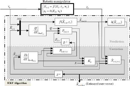
Extended Kalman filter structure
3. Biogeography-Based Optimization
BBO is a new evolutionary algorithm inspired by biogeography, which is developed by Dan Simon in 2008. It is a population-based stochastic search algorithm. Similar to other evolutionary computation algorithms, such as PSO, BBO is a search method that exploits the theory of island biogeography38,39, it is designed based on the migration strategy of (animals, fish, birds, or insects) to solve the problem of optimization. in BBO, the population represents a number of habitats (or islands), each habitat represents a possible solution for the problem at hand, and each feature of the habitat is called a suitability index variable (SIV). A quantitative performance index, called habitat suitability index (HSI), is used as a measure of the quality of a solution; which is analogous to fitness in other optimization algorithms. High- HSI habitat represents a good solution and low-HSI habitat represents a poor solution. Solution features emigrate from high-HSI habitats (emigrating habitat) to low-HSI habitats (immigrating habitat). BBO algorithm works on the basis of two concepts: migration and mutation
The migration operators, which are emigration and immigration, are used to improve and evolve a solution to the optimization problem. Migration involves two main processes immigration (λs) and emigration (µs). These parameters are affected by the number of species (s) in a habitat and they are used to probabilistically share information between habitats. Figure 2 shows the relationship between immigration rate, emigration rate. It has two main operators, which are migration (including emigration and immigration) and mutation. The immigration rate λs and emigration rate µs and the number of species (s) can be modeled as Figure 2.
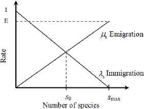
A Linear model of immigration and emigration rates38
As is clear from Figure 2 that I and E are the maximum possible immigration and emigration rates, respectively. s0 is the equilibrium number of species and smax is the maximum species number.
The immigration and emigration rates are given as
Migration operator is used to modify existing islands by mixing features within the population.
|
Migration
where NP denote population size, rand(0, 1) is a uniformly distributed random number in the interval [0, 1] and Xij is the jth SIV of the solution Xi.
Mutation operator is used to changinge SIV within a habitat itself, and thus probably increase diversity of the population. For each habitat, a species number probability
Biogeography-based optimization algorithm main steps are illustrated by the flowchart in Figure 3.
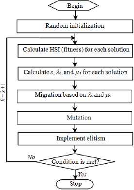
Algorithm flowchart of BBO
4. Problem formulation and proposed method
4.1. Problem formulation
The dynamic model of a robotic manipulator in the standard form can be represented by 40:
Our objective is to design a bounded control law for the input τ such that all signals are bounded and the actual state trajectories X = [θ1, θ2]T, converge to the desired trajectories Xd = [θ1dθ2d]T as closely as possible, for all time interval T = [0, tf] when t tends to infinity despite the presence of parametric uncertainties and external disturbance. Two conventional properties of the robot manipulators are considered.
Property 1
M(θ) is symmetric and positive definite, MT = M
Property 2
In respect of the dynamic system presented in (11), the following assumptions will be made:
Assumption 1
The joint positions and the joint speeds are unavailable.
Assumption 2
The disturbances d is unknown but bounded, i.e. |d| ⩽ D.
Assumption 3
The desired trajectory θd,
Assumption 4
The allowable values of the control input τ(t) are limited between an upper and lower bounds
The robustness of closed loop system against parametric uncertainties and external disturbances needs a robust control law. To attain this objective, we apply the sliding mode control approach41, this choice is motivated by its design simplicity and its high robustness against uncertainties and external disturbances.
4.2. Sliding mode control based on interval type-2 fuzzy for 2-Links manipulators
In this section, the integration of interval type-2 fuzzy logic in the sliding mode control is discussed to make an intelligent controller so-called interval type-2 fuzzy Sliding mode control based on switching gain.
For designing the proposed control law, we let the estimated tracking error:
The first step of SMC is to design the sliding surface S, which can be defined as42:
The time derivative of (14) is given as:
The Second step of SMC is to design the control law. In the traditional SMC, the discontinuous control law is selected as:
The equivalent control τeq is given by the following condition41:
In order to govern the system states to follow the desired reference trajectory just now to make S = 0 attractive. Therefore, ê → 0 as t → ∞.
A sufficient condition to achieve this behavior is to select the control strategy so that the following sliding condition41,43 is satisfied:
Consider the control problem of nonlinear uncertain system (11), the conventional sliding mode control is given as:
The use of the discontinuous sign function will excite an undesired phenomenon called chatter, which is caused by the discontinuous switching function. In this context, high switching gain K of τdis in (15) will lead to an increase in oscillations of the control torque signal, and therefore an excitation of high frequency dynamics, consequently, a chattering phenomenon will be created. Moreover, a low switching gain K can reduce the chattering phenomenon and improve the tracking performance despite uncertainties and external disturbances. However, increasing the gain causes an increase of the oscillations in input control around the sliding surface. To achieve more appropriate performance, this gain must be adjusted. This adjustment is based on the distance between the system states and the sliding surface. That is to say, the gain should be high when the state trajectory is far from the sliding surface, and when the distance decreases, it should be reduced. In the litter-ateur, various solutions can be found to overcome this problem43,12,13,14,6. In our work, interval type-2 fuzzy logic system44,45,46,47 has been used to realize this idea by combining IT2FLS with discontinuous control according to some appropriate fuzzy rules. A type-2 fuzzy logic system (T2FLS)45,46, consists of five parts: the fuzzifier, knowledge base, fuzzy inference engine, type-reducer, and defuzzifier. The knowledge base is composed of a collection of fuzzy If-then rules whose rules can be stated in a linguistic manner as follows: **********
- 1.
Calculate the weight interval of each rule:
- 2.
Compute the weighted output from all rules (type reduction) based on center of sets type reducer11
- 3.
Calculation of crisp output (defuzzification) based on arithmetic mean
Therefore, control law (18) becomes:
Therefore, it can be easily verified that (22) is sufficient to impose the sliding condition
In EKF, the determination of Q and R covariance matrices is a difficult task, especially when the corresponding noises have unknown stochastic properties. In order to avoid this problem, we will consider these matrices as free parameters to be adjusted. In the literature, Vas33 was the first who adjusted these matrices manually with trial-error method. Unfortunately, this method is a tedious task. Therefore, to overcome this difficulty and to avoid trial-error method, the authors34,35,36 have used genetic algorithms, downhill simplex, and particle swarm optimization, respectively, to optimize these matrices. In our work, we suggest using a novel optimization method for the adjusting these matrices by using the BBO algorithm37 (see Figure 4).
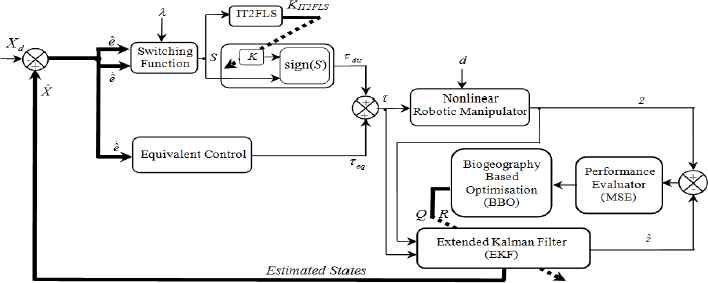
Block diagram of the control system based on the proposed BBO-EKF observer
4.3. Proposed optimized extended Kalman filter (BBO-EKF algorithm)
Estimation performance is the major problem associated to EKF; it strongly influences the parameter values of the system, state and measurement noise covariance matrices Q and R, respectively. According to Vas33, Q and R must be acquired taking into account the stochastic properties of the corresponding noises, for this reason they are generally unknown matrices. However, as these are not known, in most cases are used as weighting parameters (adjustment of parameters). Moreover, these matrices were first tuned manually by trial-error methods, which are very tedious procedures due to a large time consumption34. To avoid the computational complexity of this method, and when the values of these matrices are not known precisely, the improvement of the EKF performance can be assimilated to an optimization problem.
In this paper, we propose a novel alternative for the tuning and the optimization of Q and R based on BBO algorithm, which is described in section 3. In our algorithm, each habitat is considered as an individual and has its habitat suitability index (HSI) instead of fitness value to show the degree of its goodness. High- HSI habitat represents a good solution and low-HSI habitat represents a poor solution. Solution features emigrate from high-HSI habitats (emigrating habitat) to low-HSI habitats (immigrating habitat).
In our works, we suppose that we have a population size of NP, that xk is the k − th individual in the population, that the dimension of our optimization problem is n, and that xk(s) is the s − th independent variable in xk, where k ∈ [1, NP] and s ∈ [l, n]. At each generation and for each solution feature in the k – th individual, there is a probability of λsk (immigration probability) that it will be replaced by (7). If a solution feature is selected to be replaced, then we select the emigrating solution with a probability that is proportional to the emigration probabilities µsk in (8). Mean square error (MSE) criterion defined in (24) is used in this paper as fitness (objective function), between the actual output and the estimated one according to a certain number of iterations T to be performed for each step of estimation.
This is carried out using the two steps. As a first step, we present a BBO-EKF algorithm as in Figure 4, which is done in an offline, because BBO algorithm requires several iterations to achieve optimal solutions. For each iteration, BBO-EKF algorithm must be executed once. Therefore, BBO-EKF algorithm should be executed several times allowing the optimization of Q and R, from each measurement. The main steps of the biogeography-based optimization algorithm are illustrated in the flowchart in Figure 3, in which seven steps can be distinguished:
- 1)
Initialize a set of solutions to a problem randomly
- 2)
Calculate HSI (fitness) for each solution
- 3)
- 4)
Modify habitats (Migration) based on λs and µs, see Algorithm 1
- 5)
Mutation according to (9)
- 6)
Implement elitism to retain the best solution in the population from one generation to the next
- 7)
Go to step 2 for the next iteration if needed. This loop can be terminated after a predefined number of generations or after an acceptable problem solution has been found.
As a second step, after obtaining the optimized values Q and R in the first step, we inject them into the EKF observer running online to estimate the state variable of two-link manipulator.
The control torque input τ and the measured response z will be considered as input signals to EKF observer, where τ is applied to both robotic manipulator and extended Kalman filter (see Figure 4).
4.4. Stability of closed-loop control system
The actual output z and the estimated output ẑ are set to be the inputs of the performance evaluator of the BBO module through a comparator. The MSE is calculated by the performance evaluator. Then, obtained values of MSE will be used in the BBO algorithm. Based on these values, BBO optimizer will calculate and optimize the unknown parameters of covariance matrices Q and R.
The new solutions and updated matrices Q and R are then used to adapt the EKF for next iteration until a predefined number of iterations have been reached, and then optimal matrices Q and R are obtained. Finally, optimized Q and R are injected into EKF observer for a future online running.
In order to dominate the states of system to arrive the sliding surface s = 0 in a limited time and to stay there, the control law must be designed so that the sliding condition described in (17) is satisfied. This goal is assured by following lemma.
Lemma 1.
Consider the uncertain nonlinear system (11) and assumptions 1–4. Then, the controller defined by (22), and (23) ensures the convergence of tracking error vector to the sliding surface S.
Proof.
Consider the Lyapunov function candidate:
Its time derivative is given as:
Considering property 2, then
Combining (25)–(27), one can get
In order to obtain the stability in closed-loop, the derivative of Lyapunov function must be negative definite
Therefore, the derivative
5. Simulation and discussions
In order to verify the robustness and effectiveness of the proposed control framework, let us consider two degrees of freedom planar manipulator with revolute joints shown in Figure 5.
Two-link robot manipulator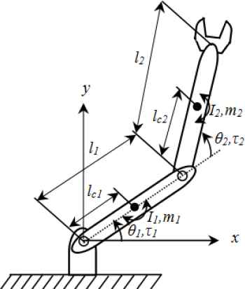
The dynamic of two-link manipulator can be described in the following differential equations38:
The matrix M0 = [mij]2×2 is given by:
The matrix C0 = [cij]2×2 is given by:
The vector G0 = [G1, G2]T is given by:
Since the Kalman filter is a discrete algorithm, then discretization of the model is needed. This discretization will be done using the forward Euler method, which provides an acceptable approximation of the systems dynamics for a short sampling period.
Let the state vector be given by
The nominal parameters of the robot used are chosen by m1 = m2 =1Kg, l1 = l2 =0.5m, lc1 = lc2 =0.25m, I1 = I2 =0.1Kg.m2, g = 9.81m/s2.
In this section, our proposed algorithm is simulated on a PC using Matlab software environment (version 8.6.0.267246). A total of T = 2000 measurement data are simulated on a time interval from 0 to 2s. Note that all codes are written in Matlab language in M-files with step size ∆t = 0.001s.
The desired reference trajectories is chosen as Xd = [70°, 90°]T . The initial values of the robot were selected as Xd = [0,0,0,0]T . Three types of uncertainties will be injected in the structure to verify the robustness of controller. Firstly parameters uncertainties (+10% over the values of nominal model parameters). Secondly the external disturbances are assumed to be time-varying as follows: δ1 = 0.3 × rand, and δ2 = 0.3 × rand × sin(t). Note that both disturbances first and second sum to d and they will be applied at t > 1s. Thirdly random Gaussian noises for the states and for the measurements both with zero mean values and with covariances q = 10−2 and r = 10−4, respectively. D = 1
EKF is implemented as in (3) to (6). The Jacobean matrices Fk, Wk, Hk, Vk are defined in appendix A; EKF will provide the state estimate vector
For comparison purposes, the performance of EKF with diverse compositions of Q and R is evaluated by using the mean-squared-error (24) of the position-estimating response, which is defined as:
First, we simulate the system under control law of traditional sliding mode action in order to show the drawback of SMC taken alone. Applying the control law (18), and after some trials, we chosen K = 20I2×2 and λ = 5I2×2, where Ii×i is an i×i identity matrix.
Table 1 shows typical EKF performance with their corresponding covariance matrices’ entries (qθ1,
| Case | Q and R entries | MSE (rad) | Estimation quality | |||||
|---|---|---|---|---|---|---|---|---|
| qθ1 |
|
qθ2 |
|
r1 | r2 | |||
| 1 | 1 | 1 | 1 | 1 | 1 | 1 | 1.0881 | Poor |
| 2 | 0.1 | 0.1 | 10−3 | 0.1 | 10−4 | 10−4 | 1.9894 × 10⁻⁵ | Good |
| 3 | 0.1 | 0.01 | 0.1 | 0.1 | 0.1 | 10−6 | 1.4567 × 10⁻⁵ | Good |
| 4 | 0.01 | 0.01 | 0.02 | 0.01 | 0.01 | 0.08 | 1.4287 × 10⁻⁵ | Very good |
EKF performances for a two-link manipulator using trial-error estimations.
The control torque inputs relative to the best case (case 4) are showed in Figure 6, where we see clearly that the control torque performance is not satisfactory due to chattering phenomenon caused by the inappropriate selection of the switching gain. In order to tackle this problem, the smoothing property of interval type-2 fuzzy logic is exploited as seen in subsection 4.2 to reduce the chattering effect.
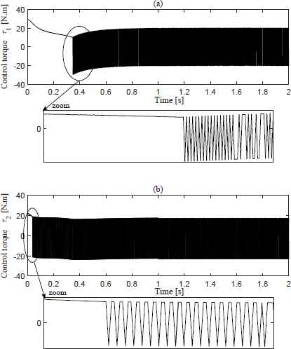
Control torque inputs using traditional SMC (a) Link-1, (b) Link-2
5.1. Chattering phenomenon problem
In this section, to avoid chattering phenomenon, one-input one-output IT2FLS is designed with an input S, which reflects the distance of error trajectory to the sliding surface. Output of IT2FLS is denoted by KIT2FLS. The memberships functions of S are chosen as illustrated in Figure 7(a), in which the following linguistic variables have been used: negative (N), zero (Z), positive (P). The memberships functions of KIT2FLS are chosen as illustrated in Figure 7(b), in which the following linguistic variables have been used: positive small (PS), positive big (PB). The rule set of the adopted IT2FLS contains 3 rules defined as following:
- Rule 1:
If S is N, Then KIT2FLS is PB
- Rule 2:
If S is Z, Then KIT2FLS is PS
- Rule 3:
If S is P, Then KIT2FLS is PB
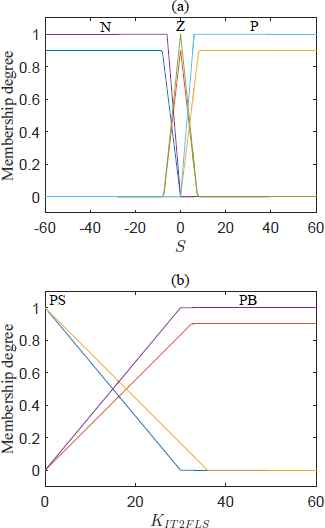
(a) Input membership functions (b) Output membership functions
These rules govern the input-output relationship between S and KIT2FLS by adopting the Mamdani-type inference engine, in which the center of gravity method is used for defuzzification as in (21). By considering the assumption 4, in which −30 ⩽ τ(t) ⩽ 30, the simulation results corresponding to improvement of switching gain K are presented using IT2FSMC with standard EKF.
Figure 8(a) shows desired, actual and estimated position of Link-1, and as we see the performance under occurrence parameter variations and external disturbance are satisfactory (see also Figure 8(b)), which represents the position tracking error of Link-1.
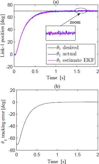
(a) Desired, actual and estimated position of Link-1 (b) Position tracking error of Link-1, using IT2FSMC with standard EKF
Figure 9(a) shows desired, actual and estimated position of Link-2, and as we see the performance under occurrence parameter variations and external disturbance are satisfactory (see also Figure 9(b)), which represents the position tracking error of Link-2. From comparing the new obtained control torque inputs in Figure 10 with the old one (Figure 6), we can clearly see that the chattering phenomenon is disappeared. The fuzzy gain KIT2FLS is depicted in Figure 11.
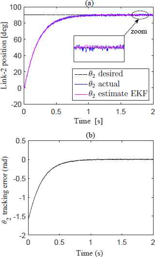
(a) Desired, actual and estimated position of Link-2 (b) Position tracking error of Link-2, using IT2FSMC with standard EKF
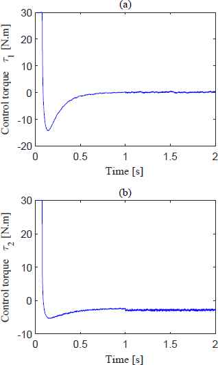
Control torque inputs using IT2FSMC with standard EKF for (a) Link-1, (b) Link-2
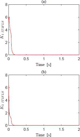
Fuzzy gain KIT2FLS obtained by IT2FLS for (a) Link-1, (b) Link-2
From simulation results, it is clear that IT2FSMC controller provides desired response with smooth control signal and minimum reaching time during model uncertainties and disturbances. Note that the prediction accuracy of EKF is not quite satisfactory (see Figures 8(a) and Figures 9(a)) due to the trial-error choice for EKF covariance matrices. In what follows, the proposed method will be applied in order to resolve the prediction problem.
5.2. Prediction problem
Note that in all above simulations, the EKF covariance matrices were adjusted by using the trial-error method, which is simple to achieve, but it takes a very longtime. Therefore, a satisfactory performance estimation can only be achieved with a larger effort by the operator experienced (experts). In fact, it is not possible to easily deduce a relationship between the covariance matrices and the best estimation results. In what follows we propose to solve this problem by a new evolutionary algorithm called biogeography-based optimization, and is then compared to PSO algorithm.
5.2.1. BBO-EKF method
In proposed method, BBO-EKF is an optimization algorithm combining the BBO algorithm with the EKF observer. We suggest searching the optimal combination of six variances qθ1,
By running the BBO-EKF with BBO parameters cited in Table B.1 (see Appendix B), the optimized covariance matrices Q and R and their corresponding performance MSEs for various numbers of iterations are given in Table 2.
| Number of Species | Generation | Q and R entries | MSE_BBO (rad) | |||||
|---|---|---|---|---|---|---|---|---|
| qθ1 |
|
qθ2 |
|
r1 | r2 | |||
| 20 | 5 | 0.0054 | 0.0484 | 0.0054 | 0.0035 | 0.0797 | 0.0666 | 5.7355 .10−6 |
| 10 | 0.0029 | 0.0696 | 0.0063 | 0.0015 | 0.0823 | 0.0960 | 4.1097 .10−6 | |
| 50 | 0.0002 | 0.0312 | 0.0302 | 0.0295 | 0.0941 | 0.0643 | 3.7545 .10−6 | |
| 100 | 0.0001 | 0.0121 | 0.0564 | 0.0188 | 0.0842 | 0.0791 | 2.7394 .10−6 | |
Optimized EKF performances using BBO algorithm.
In Table 2, the best solution is a habitat having a low MSE. We observe that the MSE is decreased to 2.7394 × 10⁻⁶ after 100 iterations. Note that this MSE is very small compared to the MSE obtained by trial-error method (MSEtrial–error = 1.4287 × 10⁻⁵), which confirm the effectiveness of proposed method.
It should be noted that the convergence of BBO algorithm to the optimal solution depends on the parameters values shown in Table B.1 (see appendix B).
In order to compare the performance of BBO-EKF process with other algorithms, we give in Table 3, performance using PSO-EKF method.
| Iterations | Generation | Q and R entries | MSE_PSO (rad) | |||||
|---|---|---|---|---|---|---|---|---|
| qθ1 |
|
qθ2 |
|
r1 | r2 | |||
| 20 | 5 | 10−3 | 0.0214 | 10−2 | 0.0632 | 0.0793 | 0.0638 | 9.8340 .10−6 |
| 10 | 10−4 | 0.0335 | 10−5 | 0.0326 | 0.0500 | 0.0832 | 9.7784 .10−6 | |
| 50 | 10−6 | 0.0772 | 10−4 | 0.0313 | 0.0673 | 0.0800 | 6.9638 .10−6 | |
| 100 | 10−5 | 0.0675 | 10−5 | 0.0157 | 0.0893 | 0.0923 | 5.1932 .10−6 | |
Optimized EKF performances using PSO algorithm.
5.2.2. PSO-EKF method
The optimized covariance matrices Q and R and their corresponding performance MSEs that have been obtained using PSO-EKF algorithm are given in Table 4 where we see that the MSE is decreased until 5.1932 × 10⁻⁶ after 100 iterations.
From the results shown in Tables 2 and 3, comparison of BBO-EKF and PSO-EKF approaches shows that all are able to find the optimum design covariance matrices Q and R. It can be easily seen that BBO-EKF gives more precise results than PSOEKF when the number of iteration (generation) increases. It can also be seen that these MSEs are very small compared to the MSE obtained by trial-error (MSEtrial–error = 1.4287 × 10⁻⁵); therefore, it can be confirmed that IT2FSMC combined with BBO-EKF technique, outperform those of PSO-EKF approach.
It should be noted that the convergence of PSO method to the optimal solution depends on the parameters c1, c2 and w, in which Self-recognition coefficient c1 = 1.49, Social coefficient c2 = 1.49, and Inertia weight w = 0.73. The comparison was carried out in the same conditions as in BBO method (initial population, Swarm size, population size).
Figure 12 shows the comparison of objective function (MSE) values for the best solutions obtained through the BBO-EKF and PSO-EKF algorithms versus the 100 iterations, respectively. The simulation results of applying IT2FLS approach with proposed optimized EKF are shown in Figures 13 to 17 were in Figure 13(a) we present the desired, actual and estimated position responses of Link-1 with optimal values of EKF covariance matrices given in Tables 1, 2 and 3 for trial-error, BBO and PSO methods, respectively. The corresponding position estimation errors are presented in Figure 13(b). The corresponding desired, actual and estimated speed and its estimation errors are presented in Figures 14(a) and (b), respectively. In Figure 15(a) we present the desired, actual and estimated position responses of Link-2 with optimal values of EKF covariance matrices given in Tables 1, 2 and 3 for trial-error, BBO and PSO methods, respectively. The corresponding position estimation errors are presented in Figure 15(b). The corresponding desired, actual and estimated speed and its estimation errors are presented in Figures 16(a) and (b), respectively. The external disturbances applied on Link-1 and Link-2, are depicted in Figures 17(a) and (b), respectively. In all these figures, we see that the best results are obtained with proposed BBO-EKF method where it can be seen that BBO-EKF fits the true state variables with higher accuracy for a two-link manipulator.
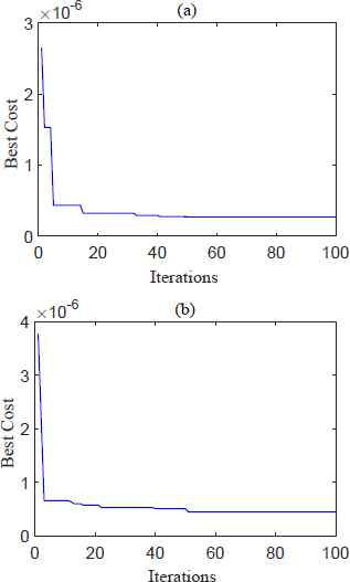
Mean-square-error comparison versus 100 iterations between (a) BBO-EKF, (b) PSO-EKF
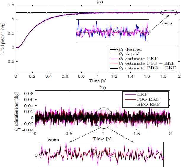
(a) Desired, actual and estimated position of Link-1 (b) Position estimation errors of Link-1, using IT2FLS SMC for different EKF optimization algorithms
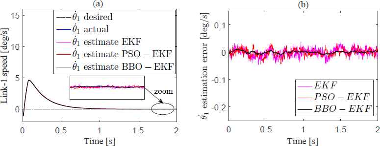
(a) Desired, actual and estimated speed of Link-1 (b) Speed estimation errors of Link-1, using IT2FLS SMC for different EKF optimization algorithms
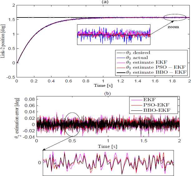
(a) Desired, actual and estimated position of Link-2 (b) Position estimation errors of Link-2, using IT2FLS SMC for different EKF optimization algorithms
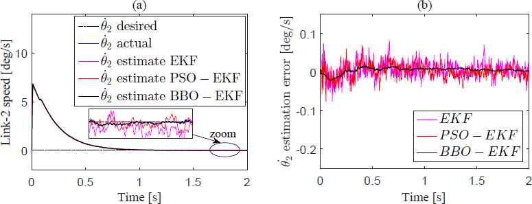
(a) Desired, actual and estimated speed of Link-2 (b) Speed estimation errors of Link-2, using IT2FLS SMC for different EKF optimization algorithms
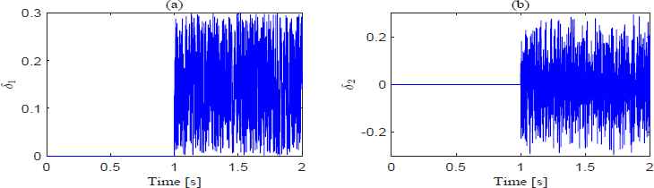
External disturbances applied on (a) Link-1, (b) Link-2
6. Conclusions
In this paper, considering parameter uncertainties and external disturbances, we have proposed a novel application of biogeography-based optimization approach for optimizing the extended Kalman filter. The interval type-2 fuzzy system was combined with sliding mode control to ensure a good robustness. The stability of closed-loop system is guaranteed by means of the Lyapunov stability criterion. The performance of EKF has been improved by adjusting parameters of the covariance matrices Q and R, in which BBO algorithm is used, and it is compared to PSO technique. The proposed optimization methods enable the noise covariance matrices Q and R, on which the performance of EKF critically depends, to be properly selected. A comparison between the IT2FSMC control combined with BBO-EKF, and with PSO-EKF were done in the presence of stochastic measurement noises, confirms that the performance of IT2FSMC combined with BBO-EKF technique was better than it combine with PSO-EKF technique. Simulation results show a significant improvement of the performance while using the proposed optimization methods to improve state variables estimation performance of the two-link manipulator and it was concluded that, the control performance of the IT2FSMC combined with BBO-EKF technique was better than it combine with PSO-EKF technique. Finally, we can say that the obtained results yield better performance while using proposed approach than traditional one.
Appendix A
Jacobian matrices Fk, Wk, Hk, Vk for a two-link manipulator
Appendix B
Parameters values used in BBO algorithm
| Parameter | value |
|---|---|
| Number of habitats (Population size) NP | 20 |
| Maximal number of generation | 100 |
| Number of decision variables (SIVs) | 6 |
| Immigration and emigration rates E, I | 1 |
| Absorption coefficient α | 0.9 |
| Probability mutation mmax | 0.1 |
BBO parameters.
References
Cite this article
TY  - JOUR
AU  - Ali Medjghou
AU  - Mouna Ghanai
AU  - Kheireddine Chafaa
PY  - 2018
DA  - 2018/03/14
TI  - BBO optimization of an EKF for interval type-2 fuzzy sliding mode control
JO  - International Journal of Computational Intelligence Systems
SP  - 770
EP  - 789
VL  - 11
IS  - 1
SN  - 1875-6883
UR  - https://doi.org/10.2991/ijcis.11.1.59
DO  - 10.2991/ijcis.11.1.59
ID  - Medjghou2018
ER  -